Do prevalence expectations affect patterns of visual search and decision-making in interpreting CT colonography endoluminal videos?

F a n s h a w e , T h o m a s R., P h illi p s, P e t er, Pl u m b , An d r e w A., H el b r e n , E m m a , H a lli g a n , S t e v e , Taylor, S t u a r t A., G al e , Ala s t ai r a n d M a ll e t t, S u s a n ( 2 0 1 6 ) D o p r e v al e n c e e x p e c t a ti o n s aff e c t p a t t e r n s of vis u al s e a r c h a n d d e ci sio n-m a k i n g in in t e r p r e ti n g CT c olo n o g r a p h y e n d ol u mi n a l vi d e o s ? B ri ti s h Jo u r n a l of R a d i olo gy, 8 9 ( 1 0 6 0 ).

Do w n l o a d e d fr o m : h t t p ://i n si g h t . c u m b r i a . a c . u k /i d/ e p ri n t/ 2 0 9 3 /

U s a g e o f a n y i t e m s f r o m t h e U n i v e r s i t y o f C u m b r i a’ s i n s t i t u t i o n a l r e p o s i t o r y ‘I n s i g h t ’ m u s t c o n f o r m t o t h e f o l l o w i n g f a i r u s a g e g u i d e l i n e s .

Any it e m a n d it s a s s o ci a t e d m e t a d a t a h el d i n t h e U niv e r si ty of C u m b r i a ’s in s ti t u ti o n al r e p o si t o r y I n si g h t ( u nl e s s s t a t e d o t h e r wi s e o n t h e m e t a d a t a r e c o r d ) m a y b e c o pi e d , di s pl ay e d o r p e rf o r m e d , a n d s t o r e d i n li n e wi t h t h e JIS C f ai r d e a li n g g ui d eli n e s ( av ail a bl e

h e r e) fo r e d u c a t i o n al a n d n o t-fo r-p r ofi t a c tiviti e s

p r o v i d e d t h a t

• t h e a u t h o r s , ti tl e a n d full bi blio g r a p h i c d e t ail s of t h e it e m a r e ci t e d cl e a rly w h e n a n y p a r t

of t h e w o r k is r ef e r r e d t o v e r b a lly o r i n t h e w ri t t e n fo r m

• a h y p e rli n k/ U RL t o t h e o ri gi n al I n si g h t r e c o r d of t h a t it e m is i n cl u d e d i n a n y ci t a ti o n s of t h e w o r k

• t h e c o n t e n t is n o t c h a n g e d i n a n y w a y

• all fil e s r e q ui r e d fo r u s a g e of t h e it e m a r e k e p t t o g e t h e r wi t h t h e m a i n it e m fil e.

Yo u m a y n o t

• s ell a n y p a r t of a n it e m

• r e f e r t o a n y p a r t of a n it e m wi t h o u t ci t a ti o n

• a m e n d a n y it e m o r c o n t e x t u ali s e it i n a w a y t h a t will i m p u g n t h e c r e a t o r ’s r e p u t a t i o n

• r e m ov e o r a l t e r t h e c o py ri g h t s t a t e m e n t o n a n it e m . T h e full p oli cy c a n b e fo u n d h e r e.

Alt e r n a t iv ely c o n t a c t t h e U niv e r si t y of C u m b ri a R e p o si t o ry E di t o r b y e m a ili n g

1

TITLE

Do prevalence expectations affect patterns of visual search and decision-making in interpreting CT colonography endoluminal videos?

SHORT TITLE

Prevalence expectations in CT colonography

TYPE OF MANUSCRIPT Full Paper

AUTHOR LIST

Thomas R. Fanshawe PhD (Corresponding Author)

Nuffield Department of Primary Care Health Sciences, University of Oxford, Radcliffe Observatory Quarter, Woodstock Road, Oxford, UK. OX2 6GG.

thomas.fanshawe@phc.ox.ac.uk

Peter Phillips PhD

Health and Medical Sciences Group, University of Cumbria, Lancaster, UK. LA1 3JD.

Andrew Plumb MRCP FRCR

Centre for Medical Imaging, University College London, London, UK. NW1 2PG.

Emma Helbren FRCR

Centre for Medical Imaging, University College London, London, UK. NW1 2PG.

Steve Halligan MD FRCP FRCR

Centre for Medical Imaging, University College London, London, UK. NW1 2PG.

Stuart A. Taylor MD MRCP FRCR

Centre for Medical Imaging, University College London, London, UK. NW1 2PG.

Alastair Gale PhD

Applied Vision Research Centre, Loughborough University, Loughborough, UK. LE11 3TU.

Susan Mallett DPhil

Test Evaluation Research Group, Public Health, Epidemiology and Biostatistics, School of Health and Population Sciences, University of Birmingham, Birmingham, UK. B15 2TT.

FUNDING AND ACKNOWLEDGMENTS STATEMENT

2

3

Title:

Do prevalence expectations affect patterns of visual search and decision-making in CT colonography?

Abstract

Objectives: To assess the effect of expected abnormality prevalence on visual search and

decision-making in CT Colonography (CTC).

Methods: Thirteen radiologists interpreted endoluminal CTC fly-throughs of the same group

of ten patient cases, three times each. Abnormality prevalence was fixed (50%) but readers

were told, before viewing each group, that prevalence was either 20%, 50% or 80% in the

population from which cases were drawn. Infra-red visual search recording was used.

Readers indicated seeing a polyp by clicking a mouse. Multilevel modelling quantified the

effect of expected prevalence on outcomes.

Results: Differences between expected prevalences were not statistically significant for time

to first pursuit of the polyp (median 0.5s, each prevalence), pursuit rate when no polyp was

on-screen (median 2.7s-1, each prevalence) or number of mouse clicks (mean 0.75/video

(20% prevalence), 0.93 (50%), 0.97 (80%)). There was weak evidence of increased tendency

to look outside the central screen area at 80% prevalence, and reduction in positive polyp

identifications at 20% prevalence.

Conclusions: This study did not find a large effect of prevalence information on most visual

search metrics or polyp identification in CTC. Further research is required to quantify

4

Advances in Knowledge: Prevalence effects in evaluating CTC have not previously been

assessed. In this study, providing expected prevalence information did not have a large

effect on diagnostic decisions or patterns of visual search.

Keywords

Colon; Colonic Polyps; Colonography, Computed Tomographic; Diagnosis,

Computer-Assisted; Visual Perception

Abbreviations and acronyms CI: Confidence Interval

CTC: CT Colonography

HR: Hazard Ratio

OR: Odds Ratio

REC: Research Ethics Committee

5

Introduction

If we are expecting an event, we are more alert to it and more likely to react when it occurs

(1). We might expect that radiologists are more alert to the presence of an abnormality

when given an indication that prevalence is particularly high and, conversely, be less alert

when the chance of encounter is believed to be low, as in screening.

Interpretation of medical imaging occurs in three environments: the symptomatic

population, the asymptomatic/screening population and the research setting. Expected

levels of abnormality vary considerably between these settings and between different

medical specialties (2). It follows that the effect of varying prevalence of abnormality on

image interpretation is crucial to our understanding of how diagnostic accuracy and

interpretative performance might change across reporting environments.

In 2011, a systematic review (3) found only three medical imaging studies (4-6) that

assessed the impact of experimentally-modified prevalence on reader diagnosis.

Subsequent studies have been published (7-10), but the relationship between prevalence

and interpretation accuracy remains unclear. Some studies report increased false negatives

or reduced diagnostic confidence at lower prevalence levels, for example for interpretation

of pulmonary arteriograms (4), mammograms (8, 11) or ankle trauma radiographs (7). This

‘rare target’ effect has also been reported in non-clinical scenarios, such as baggage

scanning (12, 13) and artificial target search experiments (14). In contrast, in chest

radiography the evidence for a prevalence effect on diagnostic accuracy is weaker (5, 9),

6

suggested a possible association between increased prevalence and the duration and

pattern of image scrutiny (10, 15).

Despite increasing use of CT Colonography (CTC) in routine practice, there is little research

describing the effect of abnormality prevalence on diagnostic performance (3). This is

surprising because CTC is commonly applied across a wide range of expected prevalences,

from asymptomatic screenees (16-18) to symptomatic and high-risk patients (19-21).

Establishing the presence or absence of a prevalence effect on reader attention, visual

search and diagnostic performance is important both in understanding how CTC should be

used in clinical practice and for designing future research studies.

The purpose of this study was to assess the effect of expected abnormality prevalence on

7

Materials and Methods

Research Ethics Committee (REC) approval was obtained to record eye tracking data from

consenting observers in this prospective study. Institutional Review Board and REC approval

was granted to use anonymous CTC data collated in previous studies (22, 23).

Participants and Cases

Thirteen radiologists (readers) were recruited from a UK training hospital over two days in

July 2012. All provided written, informed consent. Readers (6/13 male; mean age 32, range

27-36 years) were trainees with 1-7 years experience as a radiologist and at most 50 cases

CTC experience.

Ten CTC endoluminal fly-through videos lasting 30s each were generated (EH, PP) with

dedicated CTC software on a medical imaging workstation (Vitrea, Vital Images, Minnesota,

USA) and exported for viewing. Navigation speed was fixed at approximately 1.5cm/s. Five

videos depicted a single colorectal polyp (‘true positive’, 5-8mm maximal transverse

dimension), verified by three radiologists with more than 200 cases experience (23). To

counteract recall, cases were excluded if they contained polyps within five seconds

navigation of the cecal pole, rectal ampulla or insufflation catheter, or contained other

distinctive characteristics, assessed by a radiologist with six years experience (EH). Polyps

were onscreen for between 2.4 and 11.1s. The remaining five videos (‘true negative’) were

8

The sample size was based on practical considerations: the number of readers available and

the number of cases that could be assessed comfortably in one sitting. As the primary

outcome measures have not been used before in this context, no power calculation was

performed.

Data Collection

The group of ten videos was presented to each reader three times in one sitting, with an

optional break between groups. The order of cases was randomized for each reader.

Before viewing each group, readers were told that the videos in that group came from a

population with known prevalence of abnormality – 20%, 50% or 80%. The ordering of the

three prevalence scenarios was varied between readers using block randomization. Readers

were not told that the three groups actually contained the same ten videos repeated three

times, and were therefore unaware that the true prevalence was identical (50%) and the

declared 20% and 80% prevalence levels were incorrect. Information given to readers was

worded as:

“We are going to show you 3 groups of 10 videos in a random order.

Each group is taken from a different population, each with a different prevalence of

abnormality.

Before each group we will tell you the population prevalence, either 80%, 50% or

20%.”

Readers were asked to hold a computer mouse throughout and indicate with a click (‘polyp

identification’) when they saw a lesion they considered highly likely to represent a real polyp

9

or re-view videos. They were not told which videos contained polyps and were given no

feedback about their performance. Data collection took 20-30 minutes per reader.

Viewing Conditions

Reading was conducted in a quiet room with constant, ambient light. A liquid-crystal display

monitor, 1280x1024 pixel resolution, was used (SyncMaster 971P: Samsung, Suwon, South

Korea; Fujitsu E19-5: Fujitsu, Tokyo, Japan; 1 pixel=0.29mm). The screen was positioned

60cm in front of the reader. Videos measured 512x512 pixels (14.8x14.8cm), representing a

visual angle of 14.1°. Eye position of readers was recorded using a Tobii X50 or X120 eye

tracker (Tobii Technology AB, Danderyd, Sweden), sampling at 50Hz or 60Hz respectively,

positioned beneath the screen. No head-rest was used. Readers wore glasses or contact

lenses as normal. They performed a nine-point calibration procedure prior to data

collection and were excluded if this could not be completed. They then viewed a

supplemental warm-up video prior to data collection. They were not asked to fixate a

particular point before each video.

Data Preparation

Eye position data were prepared for analysis as described elsewhere (24); a summary

follows. True positive polyps were approximated using a circular region of interest (ROI),

manually overlaid onto each video frame-by-frame by a medical image perception scientist

(PP). The center and radius of this ROI were adjusted manually to match the polyp’s

transition across the screen. Within each frame, the perpendicular distance between the

recorded eye position and the edge of the ROI was calculated and used in outcome

10

edge of the ROI was considered to be within high visual acuity. For periods when no polyp

was visible, the (x,y)-eye position coordinates were retained for analysis. Coordinates

located more than 100 pixels outside the screen area were excluded as recording errors.

Outcome Measures

Eye coordinate data were used to derive three primary and six secondary pre-specified

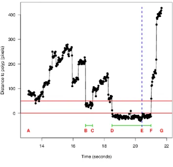
outcomes (‘metrics’); see Table 1. Figure 1 shows an example eye tracking trace (distance

between eye position and ROI over time) to illustrate metric definitions. Detailed

information about metric derivations has been reported previously (25). Metrics reflected

three aspects of reader behavior: eye position when a polyp was onscreen; eye position

when no polyp was onscreen; and frequency and accuracy of polyp identifications. Primary

outcomes were: time to first pursuit of the ROI; pursuit rate in the absence of an ROI; total

number of polyp identifications. The ‘screen coverage’ measure was defined by the

proportion of eye gaze falling into three regions: within, above or below a 256x256-pixel

square at the center of the screen. ‘Any correct identification’ and the ‘polyp on screen’

metrics are defined only for true positive videos. ‘Any incorrect identification’ is defined

only for the period before any polyp appeared, to prevent readers who delayed their

decision after seeing a polyp being misclassified as making a false positive identification.

Statistical Analysis

Metrics were analyzed using multilevel modelling, incorporating independent random

intercepts for reader and video, including prevalence level as a factor. Effects of prevalence

expectation were expressed relative to the true 50% prevalence category. In a planned

11

viewing) in which the prevalence categories were presented, this order was included as an

additional factor variable.

Within this multilevel framework, proportional hazards, logistic and Poisson models were

used, as appropriate for the data type. As most viewings had at least one missing eye

position data point, short missing data runs were imputed, based on the recorded eye

coordinates immediately before and after, and adding random measurement error.

Estimates were combined using multiple imputation methods with ten imputations (26).

Cases with more than 50% missing values or more than 50 consecutive missing values were

examined individually by two authors (TF, AP) and removed if deemed likely to make the

metric calculation highly unreliable. The Electronic Supplementary Material contains more

details.

A different approach was adopted only for pursuit rate, which has no generally agreed

definition (27). We used the number of pursuits calculated by Tobii Studio version 1.7.2

(50-pixel dispersion, 100ms minimum time threshold) throughout the period when no polyp was

onscreen, divided by the duration of this period. Time-points when the Tobii software failed

to identify whether a coordinate belonged to any particular pursuit were excluded, and the

time denominator adjusted accordingly. Cases with more than 50% missing values of the

pursuit classifier were excluded from analysis.

Results are presented as point estimates with 95% confidence intervals (95%CI) and

12

Statistical analysis used Stata 12.1 for Windows (StataCorp, College Station, TX) and R

version 3.1.1 (28).

Results

Eye tracking was successful and 389 of the intended 390 viewings were completed. Seven

(1.8%) of these were omitted from the analysis of one or more metrics (with the exception

of pursuit rate) because patterns of missing data made calculation unreliable. For pursuit

rate, 37 (9.5%) of the viewings were excluded.

Table 2 summarizes metrics across all readers within each prevalence scenario. Of the

videos that contained a polyp, readers made at least one pursuit of the polyp for 185 of the

190 (97%) viewings with reliable data.

There were no statistically significant differences between expected prevalence levels in any

metric relating to visual search while the polyp was visible (Table 3). In each prevalence

scenario, readers took approximately half a second on average to direct their gaze to the

ROI after the polyp appeared (hazard ratio (HR) 1.32 (95%CI 0.95 to 1.93, p=0.14) for 20%

versus 50% prevalence; HR 0.95 (95%CI 0.64 to 1.40, p=0.79) for 80% versus 50% expected

prevalence; Tables 2 & 3, Figure 3). Average Total assessment time span, Assessment

pursuit time and Assessment pursuit rate were also similar in the three prevalence scenarios

(Tables 2 & 3).

During the period when the polyp was not on screen, the average pursuit rate was

13

no statistically significant differences (Table 3). There was a tendency for readers’ gaze to

fall inside the central region of the screen less often at the 80% prevalence level than at the

50% prevalence level (odds ratio (OR) 0.82 (95%CI 0.72 to 0.95, p=0.008), Table 3), with a

concomitant increase in the upper region. This effect however was small, with on average

82% of gaze points falling in the central region at 80% prevalence compared to 84% at 50%

prevalence (Table 2).

There were no statistically significant differences with respect to expected prevalence

regarding the total number of identifications (Table 3). As expected, the average number of

identifications was higher for videos that contained polyps than for those that did not (1.3

versus 0.4, Table 2). The sensitivity, or probability of a polyp being correctly identified, was

higher at 50% prevalence (86%) than at 20% prevalence (71%). This difference was

statistically significant (p=0.01, Table 3) but the trend did not persist at the 80% prevalence

level (75%). This metric was subject to an extremely high case-specific effect (Figure 4), as

in three videos (1, 2 and 4) almost every reader identified the polyp at each prevalence

level; the other two videos (3 and 5), for which the polyp was superficially more difficult to

identify, are therefore likely primarily responsible for the differences in rates of correct

identification.

The probability of an incorrect identification (‘false positive’) ranged from 30% at 20%

prevalence to 39% at 80% prevalence; this difference was also not statistically significant

(Table 3). On average, incorrect identifications occurred with similar frequency for videos

that contained no polyps and for videos that contained polyps during periods when the

14

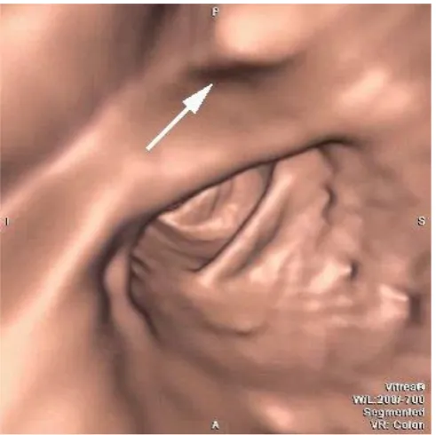
Some false positive features were identified with a mouse click by several readers (e.g. Case

3 at 5 seconds, Figures 4 and 5).

In sensitivity analysis, including as an extra factor variable the order in which the prevalence

scenarios were presented did not affect the prevalence effect sizes shown in Table 3.

Discussion

This study investigated the effect on visual search and decision-making for CTC of providing

readers with substantially different expectations of the likely prevalence of abnormality in

the population from which cases were drawn. We did not demonstrate a strong link

between prevalence expectation and the pattern of search or decision-making.

Our conclusion differs from those of several studies using scenarios other than CTC that

found increased false negative rate at lower prevalence levels (8, 12-14). Our study showed

a statistically significant increase in the proportion of polyp identifications between 20% and

50% expected prevalence, but for three reasons this finding should be treated cautiously.

First, it did not extend to the highest prevalence level, for which the proportion was similar

to that at 20%, and a non-monotonic relationship seems implausible. Second, the effect

was driven by an increased true positive rate in just two of the five cases with polyps: a

consistent increase across all cases, which would have provided more convincing evidence,

was not observed. Third, this was just one of several secondary analyses performed, and so

15

The existence of a prevalence effect is not a universal finding in image interpretation

studies. For example, Gur et al. (5) found that varying prevalence levels between 2%-21%

did not affect the diagnostic accuracy of chest radiograph assessment. Likewise, we did not

find a prevalence effect for our three primary outcomes, which were chosen to represent

visual search and decision-making. Modality may therefore be an important determinant of

prevalence effects.

We have shown previously that time to first pursuit of the polyp changes with reader

experience and the presence of a computer-aided detection marker (29, 30); in the present

study this metric was unchanged across prevalence scenarios. When no polyp was visible,

readers tended to spend more time, proportionally, looking at peripheral screen regions in

the 80% prevalence condition, but this effect is small and is not supported by changes in

other visual search metrics. However, the finding requires further investigation as our

measure is based on a simple square at the center of the screen area, which may not

adequately capture gaze narrowing effects.

We used a common set of cases for each of the prevalence conditions to directly observe

the effect of disclosing different prevalence information, as opposed to the effect of the

true case-mix. Lau et al. (31) claim that the latter may have a larger effect on

decision-making, but testing this was not our objective. Indeed, it would have been infeasible for

readers to make an assessment of the true underlying prevalence within a realistic

time-frame. It is possible that some readers realized that they had viewed videos more than

once, but this is unlikely to have a major effect on our findings: the order in which the

16

strongly associated with outcomes. Enabling all cases to be viewed with comfort in a single

sitting was an important practical consideration in our choice of the number of cases used.

Despite the number of cases being moderately small, repeated viewings of the same case

under different prevalence conditions enabled quantities of interest to be estimated with

acceptable precision.

Future studies should assess further the possibility of a threshold effect in CTC. It is possible

that the expected prevalence level needs to be lower than 20% for an effect to be visible, as

is usually the case in everyday clinical practice except in very high-risk patient groups such

as those examined following a positive fecal occult blood test (21). Evans et al. (8) found a

marked reduction in sensitivity for breast cancer diagnosis using mammography during

screening when the prevalence was extremely low (0.3%). Whether a similar effect applies

to CTC remains unknown. Additionally, prevalence effects may vary according to the ease of

visualization and identification of the cases chosen.

This study has limitations. This study was exploratory in nature, and therefore we may not

have used enough cases for subtler prevalence effects to be detected. Endoluminal

fly-through view was presented in automatic mode only, so readers could not adjust navigation

speed as in usual practice. We were therefore unable to assess the effect of prevalence on

the time the reader would spend scrutinizing each video; from laboratory experiments and

some clinical studies, there is evidence that assessment time is affected by prevalence in

static viewing modes (15, 32). Mouse clicks are not synonymous with definitive decisions

about the presence of polyps, and thus can only be regarded as proxy measures of

17

eye tracking data, it is impossible to state with certainty the cause of any particular click.

Readers were inexperienced in CTC, and so our findings are not directly generalizable to

experienced radiologists using CTC in day-to-day clinical practice. Finally, we did not assess

the effect of providing information about the spectrum of disease severity, since readers

received prevalence information alone.

In summary, CTC readers were provided with different estimates of the prevalence of

abnormalities from which cases were drawn, and study results did not demonstrate a strong

link between prevalence information and the pattern of visual search or decision-making.

Further research should investigate effects at lower prevalence levels, such as might be

present in asymptomatic populations.

Acknowledgements

This work was supported by the UK National Institute for Health Research (NIHR) under its

Program Grants for Applied Research funding scheme (RP-PG-0407-10338). A proportion of

this work was undertaken at University College London and University College London

Hospital, which receive a proportion of funding from the NIHR Biomedical Research Centre

funding scheme. The views expressed are those of the authors and not necessarily those of

18

References

1. Deese J. Some problems in the theory of vigilance. Psych Rev. 1955;62(5):359-68.

2. Kundel HL. Disease prevalence and radiological decision making. Invest Radiol.

1982;17:107-9.

3. Boone D, Halligan S, Mallett S, Taylor SA, Altman DG. Systematic review: bias in imaging

studies - the effect of manipulating clinical context, recall bias and reporting intensity. European

radiology. 2012;22(3):495-505.

4. Egglin TKP, Feinstein AR. Context bias: A problem in diagnostic radiology. JAMA.

1996;276:1752-5.

5. Gur D, Rockette HE, Armfield DR, et al. Prevalence effect in a laboratory environment.

Radiology. 2003;228(1):10-4.

6. Gur D, Bandos AI, Fuhrman CR, Klym AH, King JL, Rockette HE. The prevalence effect in a

laboratory environment: Changing the confidence ratings. Academic radiology. 2007;14(1):49-53.

7. Pusic MV, Andrews JS, Kessler DO, et al. Prevalence of abnormal cases in an image bank

affects the learning of radiograph interpretation. Med Educ. 2012;46:289-98.

8. Evans KK, Birdwell RL, Wolfe JM. If you don’t find it often, you often don’t find it: Why some

cancers are missed in breast cancer screening. PLoS ONE. 2013;8(5):e64366.

9. Nocum DJ, Brennan PC, Huang RT, Reed WM. The effect of abnormality-prevalence

expectation on naïve observer performance and visual search. Radiography. 2013;19(3):196-9.

10. Reed WM, Chow SLC, Chew LE, Brennan PC. Can prevalence expectations drive radiologists'

behavior? Academic radiology. 2014;21:450-6.

11. Gur D, Bandos AI, Cohen CS, et al. The "Laboratory" Effect: Comparing radiologists'

performance and variability during prospective clinical and laboratory mammography

interpretations. Radiology. 2008;249(1):47-53.

12. Wolfe JM, Horowitz TS, Kenner NM. Rare items often missed in visual searches. Nature.

19

13. Wolfe JM, Horowitz TS, Van Wert MJ, Kenner NM, Place SS, Kibbi N. Low target prevalence is

a stubborn source of errors in visual search tasks. Journal of experimental psychology General.

2007;136(4):623-38.

14. Rich AN, Kunar MA, Van Wert MJ, Hidalgo-Sotelo B, Horowitz TS, Wolfe JM. Why do we miss

rare targets? Exploring the boundaries of the low prevalence effect. Journal of vision. 2008;8(15):15

1-7.

15. Reed WM, Ryan JT, McEntee MF, Evanoff MG, Brennan PC. The effect of

abnormality-prevalence expectation on expert observer performance and visual search. Radiology.

2011;258(3):938-43.

16. Pickhardt PJ, Choi JR, Hwang I, et al. Computed Tomographic Virtual Colonoscopy to Screen

for Colorectal Neoplasia in Asymptomatic Adults. New England Journal of Medicine.

2003;349(23):2191-200.

17. Johnson CD, Chen MH, Toledano AY, et al. Accuracy of CT Colonography for Detection of

Large Adenomas and Cancers. New England Journal of Medicine. 2008;359(12):1207-17.

18. Stoop EM, De Haan MC, De Wijkerslooth TR, et al. Participation and yield of colonoscopy

versus non-cathartic CT colonography in population-based screening for colorectal cancer: a

randomised controlled trial. Lancet Oncology. 2011;13(1):55-64.

19. Atkin W, Dadswell E, Wooldrage K, et al. Computed tomographic colonography versus

colonoscopy for investigation of patients with symptoms suggestive of colorectal cancer (SIGGAR): a

multicentre randomised trial. Lancet. 2013;381(9873):1194-202.

20. Regge D, Laudi C, Galatola G, et al. Diagnostic Accuracy of Computed Tomographic

Colonography for the Detection of Advanced Neoplasia in Individuals at Increased Risk of Colorectal

Cancer. JAMA. 2009;301(23):2453-61.

21. Liedenbaum MH, Van Rijn AF, De Vries AH, et al. Using CT colonography as a triage

technique after a positive faecal occult blood test in colorectal cancer screening. Gut.

20

22. Halligan S, Altman DG, Mallett S, et al. Computed Tomographic Colonography: Assessment

of radiologist performance with and without Computer-Aided Detection. Gastroenterology.

2006;131(6):1690-9.

23. Halligan S, Mallett S, Altman DG, et al. Incremental benefit of Computer-Aided Detection

when used as a second and concurrent reader of CT Colonographic data: Multiobserver study.

Radiology. 2011;258(2):469-76.

24. Phillips P, Boone D, Mallett S, et al. Method for tracking eye gaze during interpretation of

endoluminal 3D CT Colonography: Technical description and proposed metrics for analysis.

Radiology. 2013;267(3):924-31.

25. Helbren E, Halligan S, Phillips P, et al. Towards a framework for analysis of eye-tracking

studies in the three dimensional environment: a study of visual search by experienced readers of

endoluminal CT colonography. Brit J Radiol. 2014.

26. Barnard J, Rubin DB. Small-sample degrees of freedom with multiple imputation. Biometrika.

1999;86(4):948-55.

27. Salvucci D, Goldberg J. Identifying fixations and saccades in eye-tracking protocols.

Proceedings of the Eye Tracking Research and Applications Symposium: ACM Press, 2000; p. 71-8.

28. R Core Team. R: A language and environment for statistical computing. Vienna, Austria: R

Foundation for Statistical Computing, 2012.

29. Mallett S, Phillips P, Fanshawe TR, et al. Tracking Eye Gaze during Interpretation of

Endoluminal Three-dimensional CT Colonography: Visual Perception of Experienced and

Inexperienced Readers. Radiology. 2014;273(3):783-92.

30. Helbren E, Fanshawe TR, Phillips P, et al. The Effect of Computer-Aided Detection Markers

on Visual Search and Reader Performance During Interpretation of CT Colonography. European

radiology.

31. Lau JS, Huang L. The prevalence effect is determined by past experience, not future

21

32. Wolfe JM, Van Wert MJ. Varying target prevalence reveals two dissociable decision criteria

22 * primary outcome

Table 1: Metric definitions. The identifying letters A, B, etc. refer to time points indicated in Figure 1.

Group Name Definition

Polyp on screen Time to first pursuit* Time between appearance of polyp (A) and start of first pursuit of polyp (B)

Total assessment time span Time between start of first pursuit of polyp (B) and polyp identification (E)

Assessment pursuit time Cumulative time in pursuit of polyp before polyp identification (B to C and D to

E), expressed as a proportion of the total time the polyp was visible (A to G)

Assessment pursuit rate Number of separate pursuits of polyp before polyp identification, divided by the

total time the polyp was visible before polyp identification (A to E)

Polyp off screen Pursuit rate* Number of distinct eye pursuits, divided by the total time when the polyp was

off screen

Screen coverage Proportion of eye coordinates falling in to each of three regions of the screen

display, ‘upper’, ‘central’ and ‘lower’; see Figure 2

Polyp identification Total number of identifications* Number of identifications recorded over whole video

Any correct identification Binary indicator of whether an identification occurred while the polyp was

visible (a reaction time of 0.5s after the polyp left the screen was allowed)

Any incorrect identification Binary indicator of whether an identification occurred before the polyp was

23

Metric 20% prevalence 50% prevalence 80% prevalence

At least one pursuit of polyp 63/63 (100%) 61/64 (95%) 61/63 (97%)

Immediate pursuit

Time to first pursuit (s) *

5/63 (8%)

0.45 [0.26, 0.65]

4/64 (6%)

0.52 [0.28, 0.82]

10/63 (16%)

0.52 [0.37, 0.95]

Total assessment time span (s) * 2.45 [1.33, 5.96] 1.75 [1.00, 3.49] 2.19 [1.15, 5.76]

Assessment pursuit time (%) 24% [14%, 34%] 21% [13%, 33%] 18% [12%, 33%]

Assessment pursuit rate (s-1) 0.59 [0.42, 0.79] 0.56 [0.42, 0.83] 0.69 [0.45, 0.85]

Pursuit rate (s-1) 2.69 [2.19, 3.09] 2.67 [2.23, 3.02] 2.71 [2.26, 3.11]

Screen coverage

Upper

Central

Lower

6% [3%, 13%]

87% [77%, 92%]

7% [4%, 12%]

7% [5%, 12%]

84% [77%, 90%]

8% [5%, 13%]

9% [5%, 15%]

82% [73%, 89%]

8% [6%, 13%]

Total number of identifications

Videos with polyps

Videos without polyps

0.75 (0.82) 1.17 (0.80) 0.34 (0.59) 0.93 (0.90) 1.38 (0.90) 0.49 (0.66) 0.97 (1.07) 1.43 (1.16) 0.51 (0.73)

Any correct identification 46/65 (71%) 55/64 (86%) 49/65 (75%)

Any incorrect identification

Videos with polyps

Videos without polyps

39/130 (30%) 21/65 (32%) 18/65 (28%) 48/129 (37%) 22/64 (34%) 26/65 (40%) 51/130 (39%) 25/65 (38%) 26/65 (40%)

Table 2: Summary of metrics by prevalence level (number (%) or median [inter-quartile

range] except for total number of identifications: mean (standard deviation)).

* Kaplan-Meier estimate, calculated without allowing for clustering, excluding viewings with immediate pursuit

24

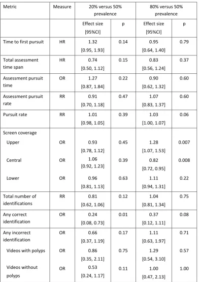
Metric Measure 20% versus 50%

prevalence

80% versus 50% prevalence

Effect size [95%CI]

p Effect size

[95%CI]

p

Time to first pursuit HR 1.32

[0.95, 1.93]

0.14 0.95

[0.64, 1.40]

0.79

Total assessment time span

HR 0.74

[0.50, 1.12]

0.15 0.83

[0.56, 1.24]

0.37

Assessment pursuit time

OR 1.27

[0.87, 1.84]

0.22 0.90

[0.62, 1.32]

0.60

Assessment pursuit rate

RR 0.91

[0.70, 1.18]

0.47 1.07

[0.83, 1.37]

0.60

Pursuit rate RR 1.01

[0.98, 1.05]

0.39 1.03

[1.00, 1.07]

0.06

Screen coverage

Upper OR 0.93

[0.78, 1.12]

0.45 1.28

[1.07, 1.53]

0.007

Central OR 1.06

[0.92, 1.23]

0.39 0.82

[0.72, 0.95]

0.008

Lower OR 0.96

[0.81, 1.13]

0.63 1.11

[0.94, 1.31]

0.22

Total number of identifications

RR 0.81

[0.62, 1.06]

0.12 1.04

[0.81, 1.34]

0.75

Any correct identification

OR 0.24

[0.08, 0.73]

0.01 0.37

[0.12, 1.11]

0.08

Any incorrect identification

OR 0.66

[0.37, 1.19]

0.17 1.11

[0.63, 1.97]

0.71

Videos with polyps OR 0.86

[0.35, 2.11]

0.75 1.29

[0.54, 3.10]

0.57

Videos without

polyps

OR 0.53

[0.24, 1.17]

0.11 1.00

[0.47, 2.13]

1.00

Table 3: Comparison of metrics between prevalence levels: hazard ratio (HR), odds ratio

25

Table and Figure Legends

Table 1: Metric definitions. The identifying letters A, B, etc. refer to time points indicated in

Figure 1.

Table 2: Summary of metrics by prevalence level (number (%) or median [inter-quartile

range] except for total number of identifications: mean (standard deviation)).

Table 3: Comparison of metrics between prevalence levels: hazard ratio (HR), odds ratio

(OR) or rate ratio (RR), as appropriate, with 95%CI and p-value.

Figure 1: Illustration of distance between eye position and polyp (edge of ROI) over time for

a single video viewing. Letters used in explanation of metric definitions, A: polyp becomes

visible, B to C: first eye pursuit of ROI, D to F: second eye pursuit of ROI, E: polyp

identification (indicated by dotted line), G: polyp disappears from view. Note short periods

of missing data at 17.7 and 19.7 seconds. The horizontal line at distance 0 represents the

edge of the ROI, and the horizontal line at distance 50 pixels the high visual acuity region

within which eye pursuits of the ROI may occur.

Figure 2: Illustration of the screen coverage metric, showing the division of the screen area

into Upper, Central and Lower regions (dashed lines). The Central region occupies a

256x256-pixel square at the center of the 512x512-pixel screen area (solid line). An

additional 100-pixel margin (shown by the outer bounding box) was allowed for gaze points

measured outside the screen area; this was incorporated into the Upper or Lower region, as

26

reader (Reader 11) viewing the same case (Case 3) under different prevalence conditions:

20% (left panel), 50% (middle panel) and 80% (right panel).

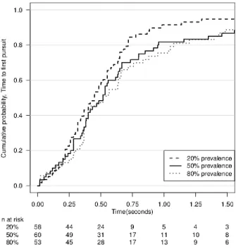
Figure 3: Kaplan-Meier curves showing time to first pursuit in the three prevalence

conditions. The vertical axis shows the proportion of viewings for which a pursuit has

occurred prior to the times shown on the horizontal axis. Below the plot, the number of

viewings per group for which a pursuit has not yet occurred is shown.

Figure 4: Time points within each video at which polyp identifications occurred. Prevalence

conditions are indicated by different colors. Cases that contain a polyp are labelled 1 to 5,

and the red bar indicates the period during which the polyp was visible on the screen. Cases

with no polyps are labelled 6 to 10.

Figure 5: Screen-capture from one of the displayed videos (Case 3, at around 5 seconds)

showing a feature provoking a false-positive, in this case a mildly bulbous but normal fold

27

Appendix A

Additional Details of Statistical Analysis

The multilevel model used for the primary analysis incorporated independent random

intercepts for reader and video and included prevalence level as a factor. If the standard

deviation of either of the random effect distributions was estimated to be zero, the model

was refitted with this random effect term removed to ensure that the estimates of the fixed

effects and their standard errors were stable. A table of estimated standard deviations of

the random effects is included as Supplemental Material.

The exact form of the model depended on the data type. A proportional hazards model was

used for two metrics (Time to first pursuit and Total assessment time span), as these are

time-to-event variables, measuring periods of time until an identification of the polyp

occurs. Only the first ‘event’ (pursuit of ROI, or polyp identification) was used for these

variables: any events occurring subsequently, such as a duplicate identification of the same

polyp or to indicate a different polyp, were discarded in the analysis of these two metrics.

Cases for which no event occurred were regarded as censored at the time the polyp left the

screen. Events that occurred at time zero, such as a reader’s gaze falling within the ROI at

the instant the polyp became visible, were excluded from the analysis as they do not

contribute to the likelihood under the standard proportional hazards model and such events

are assumed to have occurred only because of chance. The proportional hazards

assumption was checked graphically using a log-log survival plot. Results are presented as

28

Logistic models were used for variables that were binary (Screen coverage, which was

analyzed as three separate binary categories, Any correct identification and Any incorrect

identification). The metric ‘Any incorrect identification’ was analyzed separately for all

videos, for videos with polyps and for videos without polyps. This analysis was

pre-specified. The metric ‘Assessment pursuit time’, which is expressed as a proportion of the

time the polyp is visible, was also analyzed using a logistic model after first

logit-transforming the variable (a small positive value was added to observations of zero).

Results are presented as odds ratios.

Poisson models were used for the three remaining metrics (Assessment pursuit rate, Pursuit

rate and Total number of identifications). The raw counts from which ‘Assessment pursuit

rate’ was calculated showed substantial overdispersion, but this was reduced markedly by

including the appropriate time denominator as an offset, so the results are presented based

on a Poisson rather than a negative binomial model. The model for ‘Total number of

identifications’ included an adjustment for whether the case included a polyp or not,

29

Appendix B

Table: Estimated standard deviations (SD) of the case and reader random effect

distributions

Metric SD case SD reader

Time to first pursuit 0.31 0.12

Total assessment time span 0.80 0.09

Assessment pursuit time 0.31 0.38

Assessment pursuit rate 0.13 0

Pursuit rate 0.15 0.20

Screen coverage

Upper

Central

Lower

0.42

0.29

0.29

0.58

0.54

0.47

Total number of identifications 0.24 0.31

Any correct identification 3.03 0.28

Any incorrect identification

Videos with polyps

Videos without polyps

0.92

1.24

0.59

0.78

1.06

30 Figure 1