An Analysis of the Economic Impact of Strategic Deaggregation

An analysis of the economic impact of strategic deaggregation

Andra Lutu

a,b,⇑

, Marcelo Bagnulo

b

, Cristel Pelsser

c

, Kenjiro Cho

c

, Rade Stanojevic

d a_{Institute IMDEA Networks, Avda. del Mar Mediterraneo 22, 28918 Leganes, Madrid, Spain}

b

University Carlos III of Madrid, Avda. de la Universidad 30, 28911 Leganes, Madrid, Spain c

Internet Initiative Japan (IIJ), Innovation Institute, Tokyo, Japan d

Telefonica Research, Plaza de Ernest Lluch i Martin 5, Barcelona 08019, Spain

a r t i c l e

i n f o

Article history:

Received 12 December 2013

Received in revised form 8 January 2015 Accepted 10 February 2015

Available online 24 February 2015

Keywords: BGP

Traffic engineering Economics Modeling Measurements

a b s t r a c t

The advertisement of more-specific prefixes provides network operators with a fine-grained method to control the interdomain ingress traffic. Prefix deaggregation is recog-nized as a steady long-lived phenomenon at the interdomain level, despite its well-known negative effects for the community. In this paper, we look past the original motivation for deploying deaggregation in the first place, and instead we focus on its aftermath. We iden-tify and analyze here one particular side-effect of deaggregation regarding the economic impact of this type of strategy: decreasing the transit traffic bill. We propose a general Internet model to analyze the effect of advertising more-specific prefixes on the incoming transit traffic burstiness. We show that deaggregation combined with selective advertise-ments has a traffic stabilization side-effect, which translates into a decrease of the transit traffic bill. Next, we develop a methodology for Internet Service Providers (ISPs) to monitor general occurrences of prefix deaggregation within their customer base. Thus, the ISPs can detect selective advertisements of deaggregated prefixes, and thus identify customers which impact the business of their providers. We apply the proposed methodology on a complete set of data including routing, traffic, topological and billing information provided by a major Japanese ISP and we discuss the obtained results.

Ó2015 Elsevier B.V. All rights reserved.

1. Introduction

The Internet is the interconnection of over 40,000 domains known as Autonomous Systems (ASes), which engage in dynamic relationships that interplay with their technical and economic necessities. The routing between ASes relies on the Border Gateway Protocol (BGP), which is responsible for the exchange of reachability information and the selection of paths according to the routing prefer-ences of each entity active in the Internet. By tweaking BGP

configurations, network operators implement their prefer-ences in the form of routing policies, which are designed to accommodate myriad economic and technical goals. Thus, the way in which the traffic flows in the interdo-main is influenced both by the path dynamics triggered by the continuous evolution of the Internet topology and by the complexity of the routing policies of each network.

Hence, individual network managers need to perma-nently adapt to the interdomain changes and, by engineer-ing the Internet traffic, optimize the use of their network. Interdomain traffic engineering requirements are diverse and depend on the connectivity of the AS with others and on the type of business handled by the network[1]. One important task achieved through the use of traffic

http://dx.doi.org/10.1016/j.comnet.2015.02.008 1389-1286/Ó2015 Elsevier B.V. All rights reserved.

⇑Corresponding author at: Institute IMDEA Networks, Avda. del Mar Mediterraneo 22, 28918 Leganes, Madrid, Spain. Tel.: +34 91 481 6210; fax: +34 91 481 6965.

E-mail address:[email protected](A. Lutu).

Contents lists available atScienceDirect

Computer Networks

engineering tools is the control and optimization of the routing function in order to allow the ASes to shift the traf-fic inside and outside their network in the most effective way.

The injection ofmore-specific prefixesthrough BGP rep-resents a powerful traffic engineering tool which offers a fine-grained method to control the interdomain ingress traffic. This technique implies that ASes selectively announce distinct fragments of their address block to dif-ferent upstream providers. This type of phenomenon is commonly known as prefix deaggregation. For example, by using this strategy, geographically-spread networks can divert different amounts of traffic corresponding to dif-ferent points of presence (PoP), thus attracting traffic into their network through the PoP closest to the final destina-tion. Furthermore, in order to achieve load balancing pur-poses, deaggregated prefixes are announced to different providers so that the corresponding traffic flows only through the preferred transit links.

Several adjacent phenomena associated with deaggre-gation have been identified and studied by the research community. The most important negative side-effect of the widespread adoption of this technique is the artificial inflation of the BGP routing table, which can affect the scalability of the global routing system. This issue has become an important concern of the entire Internet com-munity over the past years[2]. From this perspective, this type of behavior is considered to be harmful [2], as it heavily impacts the global routing table and it acts counter to the goals of the Classless Inter Domain Routing (CIDR) architecture, which encourages address aggregation.

In this paper, we indicate that, in spite of the nega-tive overtone of prefix deaggregation, a series of advan-tageous by-products result from deploying the strategy. These by-products come up independently of the main motivation for ASes to deploy deaggregation strategies in the first place. For example, one alleged secondary

benefit is the increased security of the network

announcing more specifics in the interdomain. Some even claim that prefix deaggregation can inadvertently protect the AS against prefix-hijacking attacks [3]. Recognizing as a reality the sustained popularity of pre-fix deaggregation in the Internet [4], we look past the initial motivations behind deploying this type of strat-egy, and instead focus on its aftermath. More specifical-ly, we investigate here the potential economic impact of deaggregation, independently of the main reasons driv-ing the network operators to fragment their allocated address space.

We study the impact address-space fragmentation has on the transit traffic bill of the networks originating the more-specific prefixes, first from a theoretical point of view and then through the analysis of real-world data from an operational ISP. We find that, as a result of the unique interaction between the path dynamics in the current Internet, the asymmetrical popularity of traffic sources and the popular billing method which relies on the 95th percentile of traffic[5,6], the ASes which engineer their incoming traffic using deaggregation might enjoy one col-lateral benefit which, to the best of our knowledge, has not

been previously studied:the decrease of their transit traffic bill.1

For the purpose of this paper, we definestrategic2

deag-gregation as the action of splitting the address block and

selectively injecting each more-specific prefix to different dis-joint subsets of providers. Customers which exhibit this behavior may be able to game the 95th percentile billing rule and possibly have a negative impact on the business of their ISPs. We show that with strategic deaggregation, network operators can reduce the route diversity towards each prefix announced and, consequently, also the traffic fluctuations on the corresponding transit link, thus further impacting the monthly traffic bill paid to the transit providers.

First, we propose a model to analyze the effect of differ-ent deaggregating strategies on the traffic stability and, ultimately, on the transit cost for the deaggregating ASes. The model accounts for the route dynamics which are responsible for large traffic shifts in the interdomain, like previously observed in[7]. The general Internet model dis-encumbers our analysis of the complex Internet phe-nomena, maintaining a continuous focus on the impact of different deaggregating strategies on the transit traffic sta-bility and ultimately on the transit cost incurred on the customer ASes. We integrate in the Internet model three important elements, i.e., the interdomain routing model, the traffic model and the cost model, whose entanglement offers the necessary underlying structure for the analysis of these intricate Internet phenomena. We estimate the mod-el parameters by performing an extensive analysis of pub-licly available real BGP routing information. We afterwards quantify the actual impact of strategic deaggregation.

Second, we turn out attention to the operational Internet to detect and analyze occurrences of strategic deaggregation. We take the point of view of a transit pro-vider (with customers which might be using strategic deaggregation) and ask a two-staged question:

(1)How extensive is the use of prefix deaggregation among

the customer networks? We further propose a

methodology to identify cases of deaggregated pre-fixes within the customer base of an operational ISP within a certain time-window. We enable any operator with the necessary dataset to detect the customers which are new deaggregators and moni-tor their behavior in time.

(2)Can it be verified that deaggregation combined with

selective advertisements decreases the transit bill of some customers?

1

We stress that, in this paper, we analyze the existence of an economic

side-effectof prefix deaggregation. We do not perform here a study of the central motivations driving operators to perform prefix deaggregation in the first place, nor do we defend or encourage the usage of deaggregation in the Internet. We merely acknowledge the popularity of this strategy in the Internet and further investigate the possibility of an inadvertent economic gain for the deaggregating party. Regardless of the main goal to be achieved though deaggregation, we observe that, in certain conditions, the deaggre-gating AS can indeed enjoy a decrease of its transit traffic bill as a by-product of the deaggregation strategies deployed.

2

We propose a passive measurement approach for the detection of strategic deaggregation events and to asses their economic consequences. Our approach requires obtaining and processing private routing, topology, traffic and billing information and molding it in order to reach the correct level of understanding regarding the impact different customers might have on their providers. The novelty of this methodology is the manner in which it merges different types of information characteristic to a transit provider, in order to have a complete picture on the operations of its customer networks. Any ISP interested in detecting the occurrence of this phenomena within its customer base can construct the dataset containing all the various batches of different data and apply the pro-posed processing methodology.

The rest of the paper is structured as follows. In Section2we show the intuition behind the analyzed net-work aspects by using a toy example. In Section 3 we describe the general model for the Internet to quantify the economic impact of deaggregation techniques. In Section4we quantify the impact of strategic deaggrega-tion opposite to the case of no deaggregadeaggrega-tion. We further contrast the model-generated results with simulation and real data-driven results. We propose in Section5a novel methodology for identifying past occurrences of the deag-gregation scenario analyzed with the Internet model. In Section6we exemplify the use of the previously proposed methodology on a complex set of real-world data collected from a major Japanese ISP. We discuss in Section 7 the limitations of the proposed methodology and the chal-lenges we need to overcome when working with the real data from the operational ISP. Finally, in Section8, we con-clude the paper.

2. Toy example

Analyzing the Internet ecosystem is a challenging task, since it presents with many dynamic elements acting at different timescales. In order to achieve a better under-standing of the impact of prefix fragmentation on the tran-sit bill, we unburden our analysis of the complex Internet characteristics and intuitively present the setup we aim to analyze. We introduce next a toy example to illustrate how a network changing its strategy from non-deaggrega-tion to strategic deaggreganon-deaggrega-tion can benefit from a decreased transit traffic bill, and possibly impact the rev-enues of its providers.

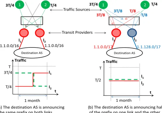
In order to clarify the main phenomena we analyze in this paper, let us consider the simple case of one destina-tion network announcing the same prefix 1.1.0.0/16 over two different transit links, like we can see inFig. 1a. We reduce the number of sources of the interdomain at two, out of which one is generating3

4of the whole trafficT

con-sumed by the destination network, and the other one, the rest. We analyze next the traffic distribution on each of the two transit links. We consider the 95th percentile pric-ing model, the most widely used method for chargpric-ing the IP transit, in which the monthly bill is the function of the peak level of traffic, not the average usage.

We monitor the level of traffic on each link during one month. We consider that source AS 1 is sending its traffic on linkl1for half of the period, after which, due to a routing

change, it starts forwarding its traffic on linkl2. Source AS 2

suffers the opposite events, namely it sends the traffic dur-ing the first half of the month through linkl2and for the

second half of the month it switches to linkl1. The transit

traffic cost is calculated using the 95th percentile rule for each of the two links. As a result, because the traffic on link

l1had a level of34Tfor more than 5% of the billing period, the

transit traffic bill for linkl1isc34T. Similarly, the transit

traf-fic bill for linkl2is alsoc34T, as for more than 5% of the

bill-ing period the traffic level was3T

4. Therefore, the total cost

paid for the consumed trafficT is c3T

2, which is with cT2

higher than the costcTpaid based on the 95th percentile rule if no routing changes would happen.

We show in this paper that, through selective deaggre-gation, the destination AS can inadvertently avoid the fluc-tuations of traffic due to routing changes and thus also decrease its transit traffic monthly bill. Consider that the destination AS divides its address space into two more-specific prefixes and announces each on a separate link, i.e. announces 1.1.0.0/17 through linkl1and 1:1:128:0=17

through linkl2, like we can observe inFig. 1b. If we assume

uniform distribution of incoming traffic for the prefix, this means that each more-specific prefix receives half of the traffic generated by each source. In this scenario, the rout-ing changes do not artificially increase the 95th percentile and the transit traffic monthly bill for the destination AS is

cT.

In the real Internet, the number of independent sources is much higher that the number assumed in this toy exam-ple. Because of this, one may think that due to the large number of sources in the interdomain, the routing changes characteristic to in the global routing system will only lead to small relative fluctuations of traffic. However, the skew-ness of the traffic distribution on sources has an important effect on the amount of traffic switching between transit links. In other words, if a large source of traffic becomes instable due to interdomain routing changes, then impor-tant amounts of traffic shift between different routes, thus heavily impacting the traffic distribution on the incoming links towards a destination.

In[8], the authors actually verify the amount of routing changes possibly affecting how traffic flows towards a des-tination. Based strictly on the information contained in public BGP routing tables, the authors go to show that those routing changes increase the transit bill of given cus-tomer with an average of 5%. Clearly, in the operational Internet some of these customer ASes are much more affected by routing changes than others. However, this average gives us a somewhat concrete idea on the manner in which the combination of routing changes, the skewed distribution of traffic on sources[9]and the popular 95% percentile billing scheme[6,5]inflate ones transit bill.

the Customer and the Provider, or even the need of the Customer to receive traffic for the more-specific locally from the Peer-Provider, thus avoiding hauling the traffic within his own network. In the scenario fromFig. 2, the Provider network also supports an additional cost implied by having to haul the customer traffic through its own net-work towards the Peer-Provider. Studying the motivation for employing this mechanism is, however, out of the scope of our analysis. We focus instead on the economic impact of deaggregation, regardless of the main reason behind deploying this strategy in the first place. In the fol-lowing section we propose a general model to analyze the savings in the monthly transit traffic bill incurred by an efficient deaggregating strategy.

3. Model description

In this section, we establish the settings of the general Internet model for the study of the impact of prefix deag-gregation on the transit traffic bill. By combining three important elements, i.e. the interdomain path changes, the 95th percentile billing rule broadly used in today’s Internet and the skewed distribution of the traffic demand on sources, the model offers the underlying structure for the analysis of the phenomena associated with the deag-gregating strategy intuitively captured by the toy example.

An initial version of this model was previously presented in[8].

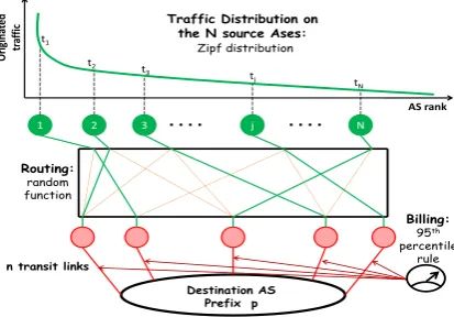
We model the Internet at the AS level, where the net-works consist of N sources and one destination AS, as we show inFig. 3. This assumption does not impact the gener-ality of our model as, in the current Internet, paths are cal-culated independently for each destination. Therefore, we focus our analysis on the case of one destination network withntransit links3 which are accommodating the traffic demand distributed overNsources in the interdomain. We assume a symmetric model where all the links have the same capacity and are equally likely to be a part of the path from a source to the destination in question. For ease of the presentation, we assume an uniform distribution of incom-ing traffic on the destination address space. As depicted in Fig. 3, we integrate three important elements in the model, i.e. the interdomain routing model, the traffic model and the cost model. Their entanglement offers the necessary underlying structure for studying the influence of various deaggregation techniques on the traffic fluctuations and the interdomain traffic bill.

Fig. 1.Toy example representation.

Fig. 2.Strategic prefix deaggregation may have additional implications in terms of costs incurred by the provider.

3.1. Deaggregation strategies and the model for interdomain routing changes

We model several different behaviors with respect to the deaggregation of announced prefixes. First, the AS can decide to announce one aggregated prefix through all its transit links. Alternatively, the AS can decide to divide the n transit links into k link sets (where k¼2; . . .; n) and announce a single more specific prefix over all the links of the set. The result is that it announces k more specific prefixes P1;P2,. . .Pk over k disjoint sets of links l1; l2; . . .; lk.

We also assume that the assigned address space can be divided evenly between the available number of link sets and announced by the destination AS as a single more-specific prefix separately on a different link set.4 Moreover, we assume that the rest of ASes in the Internet propagate the announced prefixes as injected by the origin, i.e. the other ASes honor the origin deaggregation, which is aligned with current operational practices[10]. We assume that all the announced prefixes are reachable from every AS in the Internet. This means that every AS in the interdo-main receives routes for thekprefixes corresponding to the originating AS and selects one route for each prefix.

The path selection dynamics towards the destination of interest are the result of the complex interaction between the Internet topology dynamics and the policies of differ-ent ASes along the paths between the source and the des-tination AS. The changes in the selected paths often happen as a consequence of, for example, topological modification in the network or individual routing policies changes. Usually, the timescale characteristic for these routing changes is of a few hours or days.

In order to better understand the impact of the route dynamics on the cost for transit traffic, we analyze the path changes using a timescale relevant for the billing process,

namely a month period. In particular, if we consider that the destination AS announces a given prefix Px over all the links contained in the set of links lx, we care about which ingress link of the ones contained inlxis a part of the path selected by the source AS to send traffic towards the prefixPx.

We model the BGP path dynamics towards the destina-tion of interest as follows. We define the initial state of the interdomain routing and the transitive states of the routing process in the analyzed time period. The initial state con-sists of the paths used at the beginning of the analyzed time interval by each source AS to reach the prefixes announced by the destination AS. We model this initial set of routes as a random selection between the available BGP paths between each source AS towards any destina-tion prefix. We assume that at the beginning of the inter-val, all the available transit links have the same probability of being a part of the path selected by the source AS. In other words, if a destination AS announces a prefix overxdifferent transit links, then the probability that any of those links is further a part of the forwarding path from a source towards the destination at the initial state is1

x. This implies that if the sink AS withnlinks is announcing a single prefix through all its links(i.e.k¼1), then any source AS will have to randomly select a single route in order to forward its traffic the entire address space of the destination network. If the sink AS is announcingk

fragments of the address space overkdifferent link sets, then the source AS must randomly select one path for each most-specific prefix announced (i.e.k different paths) in order to forward its traffic towards the destination AS.

In the rest of the time interval, we analyze the routing state using a time-slotted model. We divide the month into 5 min slots, which is consistent with the 95th percentile billing rule widely popular in the Internet. We encompass the dynamics of the routing process due to topology or pol-icy changes5_{by considering that in every time slot all the} source ASes are independently repeating the route selection process. We consider that with a given probabilityp the result of the random selection process is different from the initial-state path. This implies that, for a proportionp of time, traffic may shift away from the initial-state transit link towards another of the remaining equiprobable transit links. We further intent to quantify the cost paid by the des-tination AS for performing or not deaggregation in the interdomain by comparing the case in which only one pre-fix is announced over all links, thus allowing for many routing choices for the traffic sources, and the case in which a unique prefix is announced over one link only, thus strictly reducing the path diversity towards that par-ticular set of addresses. Consequently, we calculate the amount of traffic on each incoming link towards the ana-lyzed destination, while accounting for the path changes that may cause traffic to shift towards or away from the transit link.

Fig. 3.Graphical representation of the proposed Internet model.

4

Due to the manner in which the prefix can be split, this is true in the case when the number of links is equal with a power of two. In the other cases, while it is not always true that the evenly divided address space can be announced only as a single aggregated prefix, we can find a particular fragmentation of the address space that would allow us to achieve the uniformity desired and announce the smallest number of more-specific prefixes in the link set.

5

3.2. Traffic model

In this section, we analyze the traffic distribution on the available incoming links, depending on the manner the destination AS injects its prefix(es) in the interdomain. We assume that the total amount of trafficTreceived by the destination AS from the Nsources is uniformly dis-tributed across its prefixP. This means that ifTtraffic is sent toP, then if we splitPinto two more specific prefixes

P1andP2, the expected amount of traffic for each of these

more specific prefixes isT

2. In the case of an uneven traffic

distribution, it can be easily proved that a correspondingly proportional prefix fragmentation can be found such that the amounts of traffic per more-specific prefix are compa-rable. We assume that each source networkjincluded in our model generates an amount of traffictjtowards a given destination in the interdomain, as depicted inFig. 3. We assume that the generated traffictjfollows a Gaussian dis-tribution in time characterized by the statistical mean

l

j and a variance

r

2

j, which is in line with the results from [11].

3.2.1. Distribution of traffic on sources

We assume that the traffic generatedtowards one given

destination is distributed among the existing sources

according to Zipf’s law, as previously described in [12]. This assumption is consistent with the traffic measure-ments in[9], as the Zipf distribution is a particular case of a power law distribution. The Zipf distribution is one particular example of a power law[13]. A simple descrip-tion of data following such a distribudescrip-tion is the existence of a few elements that have very high values, a medium number of elements with medium values and a huge num-ber of elements with very low values (therefore, the prob-ability of larger values is very low and the probprob-ability of low values is very high). Given a ranking of the Internet entities, the Zipf law states that the traffic generated by a network is inversely proportional with its rank. For any destination network we assign the following amount of incoming traffic from AS with rankj:

tj¼

1

ja

PN

k¼1 1

ka

T¼zjT; ð1Þ

wherezjis thejranked element in a Zipf distribution cor-responding to ASj. The Zipf distribution includes a

para-meter

a

that controls the skewness of the traffic

distribution on destination networks. The total amount of transited traffic received by the destination AS can be expressed as the sum of all the traffic contributions

T¼PN_j¼1tj, for all sourcesjin the Internet.

3.2.2. Distribution of traffic on transit links

The total amount of trafficTconsumed by a particular destination AS in the Internet consists of the contribution of all the sources in the interdomain. We analyze in this section the traffic distribution on theningress links of a destination AS. We capture both the case in which the des-tination AS deaggregates to different degrees and the case

in which the AS does not fragment its address space, and we compare the results.

3.2.2.1. ‘‘No deaggregation’’ strategy analysis. We begin our

analysis by characterizing the distribution of traffic on the incoming links of a destination AS that announces its

address space as one single aggregated prefix.

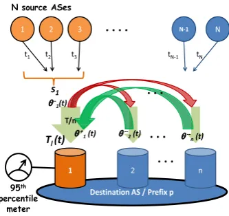
Consequently, any of the available links towards the desti-nation network can be a part of the traffic forwarding path. We include inFig. 4 an example of the traffic dynamics captured in the distribution of traffic per transit link. For a given destination AS with n transit links (each corre-sponding to a different transit provider) we define the sub-set si of sources which have as initial state path a route which includes link i, where i¼1; n. For example, in Fig. 4, subsets1includes all the source networks that have

chosen transit link 1 in the initial phase of the model. Due to the fact that each link has the same probability of being chosen by each source for traffic forwarding in the initial state of the interdomain routing process, the expected val-ue of the size of source setssiis ofNnASes. Consequently, when announcing the same prefix over all the links, the incoming traffic on each link in the initial state of the rout-ing process has a statistical expected value ofT

n.

When dividing the month in many equal-sized time-s-lots, we further consider that the route selection process happens for each source AS in every slot. Therefore, at the beginning of every time interval in the analyzed period, with a probabilitypthe newly chosen forwarding path is different from the one used in the initial state. This would trigger the shift of a certain amount of traffic from linklto the rest of the links for the destination AS and the other way around.

We denote withh_iðtÞthe random variable which repre-sentsthe traffic reductionat momenttfrom linkiand divid-ing among the rest of the transit links, as we can observe in Fig. 4. The unstable traffichiðtÞleaving linkiat momentt can be further expressed asPj2siqjðtÞtj, wheretjrepresents the traffic generated by source ASjand has the expression in(1),sirepresents the set of sources with initial-state path including linkiandqjis either 1 if at momenttlinkiis a part of AS j’s forwarding path or 0 in the contrary case. Formally,

Pðqj¼1Þ ¼p;

Pðqj¼0Þ ¼1p: ð2Þ

The traffic reduction follows a Binomial distribution, i.e.

h_i BinomialN

n;p

, withi2 ½1;n. Thus, the mean and vari-ance of the unstable traffic leaving a link, i.e.h_iðtÞwith

i¼1; n, has the following expression for any of thenlinks:

~

l

i¼p

T n; ~

r

2

l ¼pð1pÞ X

j2si t2

j: ð3Þ

When analyzing the traffic on a link we also have to considerthe traffic increasein the current linkifrom receiv-ing traffic from the rest of the linksk–i. This represents only a fraction of the total traffic moving away from any other link towards the current transit link. We denote with

the case of linki, we can expresshkðtÞas

P

j2skqjðtÞtj; k–i, whereqjis either 1 or 0 depending if at momenttlinkiis a part of the forwarding route used by the source AS or not andtjhas the expression in(1). The traffic shift probability is equal to the probability of path change p, i.e.

Pðqj¼1Þ ¼p. The total unstable traffic is represented by

P

k–ihkðtÞ. This amount evenly splits between all the

n1 equiprobable alternative links, including the ana-lyzed linki. Consequently, the expected value ofthe

incom-ing trafficdenoted byhþ_iðtÞon linkiis represented by the

1

n1part of all the total unstable traffic, i.e. 1

n1 P

k–ihkðtÞ. This random variable also follows a Binomial distribution, as it represents the addition of n1 independent Binomially distributed random variables.

We can now express the total volume of traffic on each link towards the destination, which changes at every time-slottlike showed in the following expression:

TiðtÞ ¼

T nh

iðtÞ þh

þ

iðtÞ; ð4Þ

wherehiðtÞrepresents the traffic leaving linkiandhþiðtÞ represents the expected value of the traffic shifting from the rest of the links to linki.

Therefore, the expressions for the statistical mean and variance for the total traffic on linkiwhen a single prefix is announced over all the available links are:

r

2

i ¼pð1pÞ 1 1 ðn1Þ2

! X jsij¼Nn

j2si t2

j þ 1 ðn1Þ2

XN

j¼1

t2 j 2 4 3 5;

l

i¼

T

n: ð5Þ

3.2.2.2. ‘‘Strategic deaggregation’’ strategy analysis. When

the destination AS deaggregates the assigned address block into k more-specific even prefixes, where k6n, and announces them over different link sets, different parts of the address space are reachable only through the corre-sponding subset of incoming links. Consequently, the source ASes split their traffic evenly for the deaggregated prefixes and choose one path for each fraction of the

address space. The size of the set of source ASes with an initial path including one of the incoming links towards a destination prefix is equal tojsij ¼kNn. These sources do not send all their traffic on the chosen link from a given link set, but they only send the corresponding fraction of traffic towards the destination prefix, namelytj

k.

When the destination AS deaggregates its address block in a number of prefixes smaller than the number of avail-able transit links, we haveksets of links including then

k

dif-ferent links. Consequently, the amount of traffic on each transit linkTiat timethas the following expression:

TiðtÞ ¼

T=k

n=kh

iðtÞ þ 1 n k1

X

j–i

hjðtÞ: ð6Þ

The unstable traffic from linkito the othern

k1 links in

the same set is now h iðtÞ ¼

Pjsij¼kN n j2si qjðtÞ

tj

k, where jsij ¼knN represents the number of sources in the source set si, directly proportional with the number of announced pre-fixes in the interdomain. We observe that, while the mean value of the incoming traffic remains the same as in the previous case, i.e.

l

l;k¼pTn, the expression of the traffic variance becomes:

r

2

i;k¼pð1pÞ 1 k2

1

nk

2!js_Xij¼kN

n

j2si t2

j

þpð1pÞ 1

nk

2_XN

j¼1

t2

j: ð7Þ

When evaluating the traffic variance with the expres-sion in(7) relative to the one in(5) we observe that as the number of announced prefixes k is increasing, the amount of traffic on each link becomes more stable, as its standard deviation is decreasing. This phenomenon is explained by the fact that, as the number of prefixes increases, so does the number of disjoint link sets. We have observed that in the case where only one prefix is announced over all links, there is only one link set includ-ing all the available transit links. Contrariwise, when announcing more prefixes, the number of link sets is increasing, also implying that the amount of incoming traf-fic and the number of different links included in each set are proportionally decreasing. This further translates into a decreasing number of routing choices for the traffic to reach the more-specific prefix announced on a specific link set.

3.2.2.3. The impact of strategic deaggregation. Comparing

the two expression from(5) and (7), we obtain the follow-ing ratio between the two variances:

c

¼ n1

nk

2 1þ

nk k

2

1

h i Pjsij¼kN

n j2_si t

2 j

PN

j¼1t 2 j

1þ ðn1Þ21 P

j_sij¼N n j2si t

2 j

PN

j¼1t 2 j

: ð8Þ

For 26k<nand approximatingPjsij¼knN j2si t

2

j k

Pjsij¼N n j2si t

2

j, we conclude that

c

<1, which indicates that when the degree

of deaggregation is increasing, the variance of the traffic on a link is smaller. This results in a diminution of the traffic burstiness and even smaller fluctuations in the total amount of chargeable traffic.

In the extreme case when the AS is announcing a num-ber of more-specific prefixes that is equal to the numnum-ber of transit links, the size of the set of sources with a route that includes linkiin the initial state isjsij ¼N. In other words, every source AS installs in its routing table a stable path for each transit link for the destination AS. This implies that the traffic shifting from one link to the others is zero and, similarly, the traffic incoming from the rest of the links is also null. Therefore, the variance of the traffic on each link resulting from route changes is approximatively zero

r

2

i ¼0, as the traffic forwarding paths are very stable. Consequently, the incoming traffic on each link equal with T

ndoes not fluctuate during the analyzed period, as this amount of traffic is confined to the preferred incoming link.

3.3. The cost model

The 95th percentile rule is currently the most widely-spread billing method among ISPs[6]. This method usually implies that the agreed billing period (usually a month) is sampled using a fixed-sized window, each interval yielding a value that denotes the traffic transferred during that period. The resulting intervals are sorted and the 95th per-centile of this distribution is used for billing [6]. Consequently, this billing method is considered as a com-promise between billing a customer based on the absolute traffic usage or based on the capacity of the transit links and the peak rates.

A recent transit cost survey [14] has shown that the price per unit of transfered traffic, denoted here by ct, decreases with the increase of the expected volume of transit traffic following a convex dependency. However, this is only true when the increase of the expected amount of traffic significant i.e. one order of magnitude. In the case where the increase of expected traffic volume is in the same size range as the initial traffic volume, the cost per traffic unit remains constant. We assume that the varia-tions in traffic do not change the order of magnitude of the received traffic, therefore we can also assume a linear cost function for the transit traffic.

In our model we include a cost function with the fol-lowing expression:

C¼ctV; ð9Þ

whereVis the charging traffic volume (i.e. the 95th per-centile of the monthly traffic) of the destination ASiand

ctis the corresponding transit traffic unit cost. We consider that the total charging traffic volume for any destination AS, represents the addition of all the chargeable traffic volumes on each incoming link, and therefore can be expressed as

V¼X n

i¼1

l

iþ1:96

r

i

; ð10Þ

wherenrepresents the number of incoming link for the destination AS, and

l

i and

r

i have the expressions from

(5). Given the fact that the traffic on link l follows a Binomial distributionBðN;piÞ, we can approximate it with

a Normal (Gaussian) distribution Nð

l

i;

r

2iÞ. The expression

l

þ1:96

r

from (10) represents the estimation of the 95th percentile of a Normal random variableNð

l

;

r

2Þ rep-resenting the individual traffic volume on the incoming links.

In order to capture the full impact of deaggregation on the transit traffic bill, we focus on the amount of charge-able traffic in the two extreme cases: (i) no deaggregation:

k¼1, (ii) strategic deaggregation:k¼n. We calculate next the total amount of chargeable traffic on each link, i.e. the 95th percentile of the link traffic, when no deaggregation is performed by the destination AS, i.e

v

ijk¼1and when the

number of prefixes announced is equal to the number of available links, i.e.

v

ijk¼n:

v

ijk¼1¼ T

nþ1:96

ffiffiffiffiffiffiffiffiffiffiffiffiffiffiffiffiffi pð1pÞ

p ffiffiffiffiffiffiffiffiffiffiffiffiffiffiffiffiffiffiffiffiffiffiffiffiffiffiffiffiffiffiffiffiffiffiffiffiffiffiffiffiffiffiffiffiffiffiffiffiffiffiffiffiffiffiffiffiffiffiffiffiffiffiffiffiffiffiffiffiffiX

j2sit

2

jþ 1 ðn1Þ2

X

k–i

X

j2skt

2

j

s

;

v

ljk¼n¼

T

n: ð11Þ

We can easily observe that the additional traffic on each link is

c

i¼

v

ijk¼1

v

ijk¼n

¼1:96pffiffiffiffiffiffiffiffiffiffiffiffiffiffiffiffiffipð1pÞ

ffiffiffiffiffiffiffiffiffiffiffiffiffiffiffiffiffiffiffiffiffiffiffiffiffiffiffiffiffiffiffiffiffiffiffiffiffiffiffiffiffiffiffiffiffiffiffiffiffiffiffiffiffiffiffiffiffiffiffiffiffiffiffiffiffiffiffiffi X

j2sit

2

jþ 1 ðn1Þ2

X k–i

X j2skt

2

j s

: ð12Þ

Furthermore, the difference in the total charging traffic volume for the analyzed destination AS withnlinks can be expressed as the sum of the traffic fluctuations in all the links, i.e.V¼Pn_l¼1ð

v

ijk¼1

v

ijk¼nÞ. This yields the following expression for the total volume of additional chargeable traffic:

c

¼X

i

c

i: ð13Þ

The savings in transit traffic bill represent the costcpaid for the bursty, unstable traffic. Consequently, the addition-al cost emerging from path instability in the interdomain is

c¼

c

ct: ð14Þ

Henceforth, the saved amount in the transit traffic bill rep-resents a fraction of

RS¼

c

Tþ

c

ð15Þ

out of the actual price paid for the consumed traffic with-out deaggregation. Substituting the generated traffictjfor every source AS of rankjwith the expression in(1)yields that the relative transit traffic savings are a function of the number of links towards the destination AS, the instability probabilitypand the Zipf distribution skewness parameter

a

, which does not depend onT:RS¼fðn;p;

a

Þ.

4. Numerical results and model validation

simulations and data driven estimations using real BGP traces.

In order to apply the proposed model to the current Internet and estimate the potential savings in the transit costs, we need first to assign realistic values to the model parameters, namely, N; n;

a

and p. Parameter Nstands for the number of ASes in the Internet, which is in the order of 36,000. The skewness parameter

a

for the Zipf distribu-tion on the traffic sources is estimated in the current state of the art[15,12]to a value of 0.9. As parameterp repre-sents the probability of a change in the ingress link used by the source ASes to send traffic towards the destination, we estimate it by analyzing the data set containing real BGP routing information. Parameternrepresents the num-ber of transit links which we estimate in the next section following the routing data analysis.

4.1. Data set

The data set used includes the full BGP routing table snapshots taken every 8 h from 66 different ASes present

in the RIPE database [16], during the months of

December 2010 until May 2011. This adds up to a total of more than 35,000 snapshots of full routing tables, con-taining the BGP routing information from the 66 analyzed sources towards more than 350,000 destination prefixes. We approximate the amount of traffic generated by each source by extracting from the Zipf distribution of traffic on the 36,000 sources only the elements corresponding to the official ranks for the set of 66 different analyzed sources. We use the official CAIDA ranks assigned based on the data-set from January 2011[17]. We estimate the number of different transit links per destination by identi-fying the unique second last-hops6 _{(2LH) in the paths} installed in the routing tables. We find that more than 93% of ASes have at most 7 transit providers.

4.2. Estimation of the instability probability

In order to estimate the transit link instability probabil-ity, we further observe the changes in the 2LHs of the AS paths towards the destination prefixes in the analyzed routing tables. For each source–destination AS pair, we cal-culate the probability that in a given interval the source AS is not using the link selected in the initial state towards the same prefix. For each of the 66 sources analyzed, we eval-uate the relative time the source AS is not using the path announced in the first time slot of the analyzed period towards every destination prefix. Next, we match every destination prefix to the originating AS and average the time spent on an alternative path for all the prefixes announced by the destination AS. We thus obtain the prob-ability that a source uses a path towards each destination AS which is different than the initial one. This implies that, for a proportionpof time, traffic may shift from the initial-state transit link towards another of the remaining equi-probable transit links. We approximate the parameter p

with the mean value of the transit link instability probabil-ity over all the observed sources, yielding a value of

p¼3:5%.

4.3. Savings quantifications using the analytical model

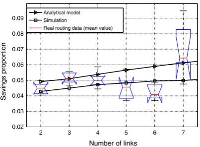
We observe inFig. 5the model savings estimated for a destination AS depending on the number of links. We con-sider an instability probability ofp¼3:5%in the interdo-main and a Zipf distribution of traffic with 36,000 elements and

a

¼0:9. We observe that a destination AS with n2 ½2;7 transit links may have an additional cost incurred by the route instabilities in the interdomain that can reach up to 6.5% of the transit traffic.

According to the results presented inFig. 5, the average value of the savings for an AS with 2 transit links, repre-senting 40% of all the ASes, is equal to 4.9% of the usual transit traffic bill.

4.4. Model validation through simulation

In order to check the accuracy of the results obtained analytically, we simulate the proposed model for a destina-tion AS withn2 ½2;7transit links. We consider that the destination AS receives traffic from 36,000 source ASes, fol-lowing a Zipf distribution with skewness parameter

a

¼0:9. We evenly divide the Internet traffic signal in 100 equal-sized time-slots for which we define the sample value of the traffic level, which is consistent with the num-ber of routing snapshots we have during a month. We con-sider that in the first time-interval, each source AS uniformly chooses one of thenproviders. In the remaining time-slots we simulate the sticky BGP selection algorithm by conceding a probability 3.5% of a different incoming link to be more appropriate for the source network than the ini-tially chosen one. We define the 95th percentile value for traffic on each transit link based on the values obtained through simulation. We apply next the formula in(15)to evaluate the savings due to the use of full deaggregation.

We represent inFig. 5the curve of the average values of savings (estimated with less than 1% margin of error at 95% confidence level) for a destination withn2 ½2;7links. We thus observe an average value of 4.3% of the transit traffic bill savings for a destination AS with 2 different transit links.

The difference between the analytical model and the simulation comes from the fact that the analytical model uses for the 95th percentile the Normal-based approxima-tion confidence interval, i.e.

l

þ1:96

r

, while this does not occur in the model simulation. In the latter case, we already have all the samples of the discrete Binomial Distribution, for which we can easily define the 95th per-centile of the link traffic level.

4.5. Savings quantification using real routing data

In this section we contrast the previously estimated numerical values for the transit link instability costs with approximations performed based on actual routing infor-mation. For this purpose, we process the BGP routing data present in the RIPE database corresponding to 6 months, 6

Thesecond last-hopis the AS which we see before the destination AS in

theAS-PathBGP attribute and it represents the upstream provider used by

from December 2010 until May 2011 generated by 66 dif-ferent sources. From comparing the routing tables we can evaluate the actual amount of routing changes towards a given destination AS in the Internet. Consequently, the path changes described bypare here substituted with gen-uine path changes inferred from comparing the routing tables over 6 months time. In our data analysis, we do not account for routing changes which are due to failures in the ingress links, since any operationally viable deaggre-gation strategy must support backup links. In order to filter out these cases, we remove from our analysis the destina-tions with a non-constant number of transit links present in each monthly data set. This approach is likely to remove a superset of the ingress-link failure cases, making our result to be only alower boundof the potential savings.

When performing the reality based approximation of the savings, the Binomial approximated distribution of traffic is no longer needed, as we can infer the amounts of traffic on each link from evaluating the actual contribu-tion of each source on every link. From the Zipf distribucontribu-tion with 36,000 elements and

a

¼0:9, we extract only the 66 elements corresponding to the sample of ASes.

We find that the amounts of savings are consistent over the 6 months, thus pointing out that the routing changes do impact the traffic levels in the same proportion each month. InFig. 5we observe the savings estimated with real routing data for the destination ASes withn2 ½2;7transit links. The boxplot for each case shows the savings over the 6 months, where the central mark is the median, the edges of the box are the 25th and 75th percentiles, the whiskers extend to the most extreme data points not considered outliers. With 95% confidence level, the average amount of savings for an AS with 2 upstream providers lies in the confidence interval½4:2%;4:77%, which is consistent with the previous approximations.

5. Strategic deaggregation detection methodology

In this section, we propose a methodology to identify real-life strategic deaggregation scenarios, which we previ-ously analyse using the model proposed in Section3. We show here how any ISP can monitor the amount of

deaggregation generated by its customers and quantify the impact strategic deaggregation may have on its own revenues. The central reasons for the customer network operator to deploy the deaggregation strategy in the first place is usually manifold and may or may not be related to decreasing the transit traffic bill. The transit provider, however, might be impacted by its customers’ choices in terms of deaggregation. As we previously show in Section3, the unique interaction of three important char-acteristics of the current Internet, namely the interdomain path changes, the 95th percentile billing rule broadly used in today’s Internet and the skewed distribution of the traf-fic demand on sources, make if possible for networks to inadvertently decrease their transit traffic bill using strate-gic deaggregation. We further argue that, by simply detect-ing the cases of strategic deaggregation, a transit provider can identify the customers who may unknowingly impact in a negative way its revenues. Furthermore, detecting a large number of such cases in ones customer base might provide the necessary incentives for the adoption of a more suited billing model than the sub-optimal 95th percentile billing rule.

We propose a passive measurement approach for the detection of strategic deaggregation events and to asses their economic consequences. The novelty of the approach is the manner in which it merges different types of infor-mation characteristic to an ISP in order to have a complete picture on the operations of its customer networks. This requires obtaining and processing routing, topology, traffic and billing information and molding it in order to reach the correct level of understanding on the economic impact dif-ferent customers might have on their transit providers. Any ISP interested in detecting the occurrence of this phe-nomena within its customer base can employ the proposed methodology.

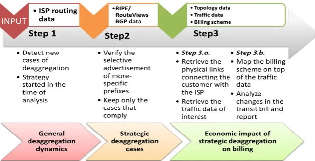
The methodology is structured in three parts, each con-veying relevant results concerning deaggregation dynam-ics within the customer base of a transit provider. We summarize inFig. 6the steps taken in the methodology and show which type of information is required for each part.

Step 1: Detect more-specific prefixes. First, we detect

ASes which change their behavior and start using deag-gregation within a predefined time-window. For this step we require the BGP routing information from the ISP (i.e., the global BGP routing table from the transit provider), as depicted in the first processing block in Fig. 6. We expand on the mechanism in Section5.1.

Step 2:Detect strategic deaggregation. Second, we check

for selective advertisements of the more-specific prefix-es previously identified. As depicted in the second pro-cessing block fromFig. 6, in this step we use all the BGP routing information from the monitors active in the RIPE RIS and RouteViews projects.

Step 3:Evaluate economic impact. Third, we try to

deter-mine if performing strategic deaggregation leads indeed to economic benefits for the customer network. For the cases of strategic deaggregation, we monitor the traffic data both (i) before deaggregation, when the address block is injected as one prefix to all providers (i.e. no

2 3 4 5 6 7

0.02 0.03 0.04 0.05 0.06 0.07 0.08 0.09

Number of links

Savings proportion

Analytical model Simulation

Real routing data (mean value)

deaggregation) and (ii) after the strategic deaggregation, when the address block is fragmented into as many more-specific prefixes as the number of transit provi-ders and each more-specific is selectively advertised to a different provider (i.e. strategic deaggregation). It is important to capture both these states, in order to be able to correctly quantify the economic impact of strategic deaggregation. We evaluate the transit bill for each case and compare. This is depicted in the third processing block fromFig. 6.

Step 3.a: We extract the traffic data on all the links

con-necting the provider with the identified customer which is deploying strategic deaggregation. This requires a previous mapping between customers and transit links from the ISP. We obtain this topology data after parsing all the router configuration files provided by the ISP. This step is further depicted in the first sub-block of the third processing block inFig. 6.

Step 3.b:Finally, we move toestimating the bill for the

aggregated and deaggregated traffic patterns. Thus, by

applying the ISP’s billing scheme to the traffic traces, we can quantify the impact of strategic deaggregation on the transit traffic bill. This step is depicted in the last processing block inFig. 6.

The methodology is aimed at working with a large and diverse collection of real data. Any ISP interested in detecting the occurrence of this phenomena within its customer base can build the dataset and employ the proposed methodology. Moreover, the tools we have developed are publicly available7 _{for the research} community.

5.1. Detection of deaggregation events

The detection algorithm we propose inStep 1for the identification of more-specific prefixes performs a com-parative analysis of the BGP information obtained from

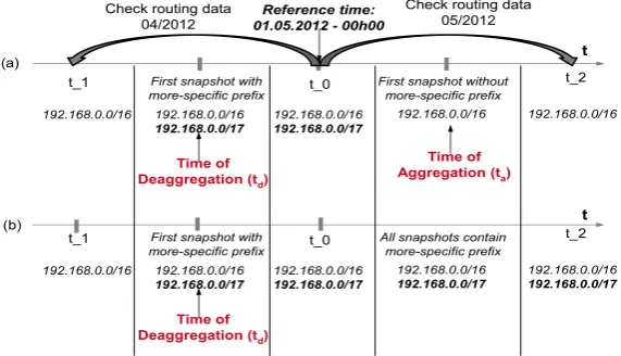
the ISP. The different states of the algorithm are depicted inFig. 7. We begin by choosing areference routing table. The time-stamp of the reference routing table represents

thereference time. The detection algorithm identifies the

customer prefixes based on the information from the pro-vider (for example, customer routes are tagged with speci-fic informational communities). We assume deaggregated prefixes exist at the reference time and we verify if the more-specific prefixes started to be advertised within the month prior to the chosen reference time. We progressive-ly contrast the content of the reference routing table with each of the previous routing tables collected for a certain period before the reference time. As depicted in Fig. 7, we verify the routing information from as much as one month before the reference time in order to capture the dynamics of prefix deaggregation in a timescale that is consistent with the billing period. The analysis of the pre-fixes advertised by the customer ASes during this par-ticular time-window allows us to separate the newly

injected more-specifics prefixes, which first started to be

injected in the month prior to the reference time. It further separates this cases in more-specifics that are not active for at least one months post-deaggregation (i.e., the situa-tion depicted inFig. 7(a)) and, contrariwise, more-specifics that are active for one month post-deaggregation (i.e., the situation depicted in Fig. 7(b)). This also enables us to determine the presence of a covering prefix injected by the customer network and the approximative moment of deaggregation.

The algorithm can be run on longer timescales (e.g. two months, three months, one year etc.), thus allowing the ISP to get a bigger picture on the deaggregation dynamics within its customer base at different timescales.

5.1.1. The two-by-two routing tables comparison

We contrast the entries from the reference routing table with any other routing table collected in the period of ana-lysis, to which we further refer as apairrouting table. We begin by first defining the set of prefixes presentonlyin the reference routing table by separating the prefixes

Fig. 6.The methodology steps: at each step we require a different input dataset depicted at the top of each processing block. At the bottom of each block, we can see the results we obtain at each step.

7

advertised only at the reference time and not present in the pair routing table, i.e.

D

i¼PrefPi ð16Þ

wherePref represents the set of prefixes in the reference

routing table andPi, the set of prefixes installed in the paired routing table. For each of the prefixes in theDiset defined above, we use a digital tree search[18]to identify the covering prefixes among the entries in the pair routing table. Assuming that no network is less specific than a=8, we are thus able to rapidly build the covering digital tree corresponding to each of the prefixes of interest. From each tree, we retrieve the least-specific prefix, i.e. the tree root, which we further use in the traffic data analysis. We do not examine the intermediate prefixes (shortly appearing intermediate phases in the deaggregation process), since for these there exists a more-specific prefix which can influence the manner in which traffic flows towards the destination.

By performing this comparative study using all the peri-odically collected routing tables from the ISP, we obtain an accurate picture of the evolution of the prefix deaggrega-tion dynamics within the customer base of the provider. We monitor the changes of the previously defined prefix sets Di during the analysis interval. The approximative time of deaggregation is, at the latest, the collection time of the first routing table snapshot which contains the can-didate more-specific route known to already be installed in the reference routing table. This moment is marked in the time-line depicted inFig. 7as the first moment where the more-specific prefix and the covering prefix are both pre-sent in the pair routing table.

5.2. Sifting the results

In order to correctly identify the long-lived deaggrega-tion events which may have an economic impact, we need to make sure that the retrieved more-specifics are not spo-radic events. We discard from our analysis the cases of

prefixes which, as depicted inFig. 7(a), get re-aggregated in their less-specific covering prefix shortly after the deag-gregation was performed. What we are interested to ana-lyze further are cases of deaggregation which match the setting inFig. 7(b), where the more-specific is active for a month after the time of deaggregation.

We apply the same detection algorithm to identify potential re-aggregation cases of more-specifics into their covering prefixes which might happen in the month after the moment of deaggregation. We perform this latter step in order to assure that from the results provided by the algorithm we select only the more-specific prefixes that remain installed in the routing table for at least one month from the moment of deaggregation, and thus may impact the transit traffic bill. For avoiding cases of dynamic deag-gregation–aggregation behavior, we filter out prefixes with intermittent presence in the routing tables, i.e. with a pres-ence time lower than 5% of the billing period.

Past the reference time, the previously described two-by-two comparison algorithm actively detects cases of re-aggregated more-specific prefixes in the Di set. We approximate the time of re-aggregation with the collection time of a pair routing table which contains only the cover-ing prefix after the reference time.

5.2.1. Validation of selective advertisements

The selective advertisements validation process is fur-ther integrated in Step 2. We combine the internal routing view from the ISP with the external views taken from the ASes participating in the RIPE RIS and RouteViews project. In particular, we identify all the active providers used for reaching both the covering prefix and the more-specific prefix from Step 1.

We aim to check if the covering prefix is injected to all the active providers and the deaggregated prefix is selec-tively injected. To this end, we analyze all the routing information retrieved during the corresponding time peri-od (one month prior to the moment of deaggregation and one month after) from all the monitors whose routing

tables we were able to retrieve from the public collectors. We monitor the routing information from each external AS towards the customer prefixes. Thus, we can infer the approximative number of active transit providers for the destination prefix by identifying the list of uniquesecond

last-hops(2LH) in theAS-PathBGP attribute after

remov-ing AS-Path prependremov-ing. The 2LH is the AS which we see before the destination AS in theAS-Path. This represents the provider used to reach the destination from the traffic source (i.e for some of the paths, this 2LH should be the ISP providing the data for this study).

We accept a certain error in the inferred connectivity degree of each customer, since we only have partial infor-mation on the interdomain routing. Given that the number of monitors active within the RIPE RIS and RouteViews pro-ject is limited[19], we have only a partial picture of how external sources of traffic reach the interest prefixes. However, since the sample of monitors is biased towards large Tier-1 networks, we assume that this is a reasonable approximation. We discuss how it influences our results, along with other limitations of the methodology in Section7.

6. Applying the proposed methodology

In this section, we show how we can apply the proposed methodology on real data obtained from an operational major Japanese ISP. The network dataset includes BGP routing tables, traffic data, topology data and the billing scheme from the ISP looking to monitor the behavior of its customers. The analysis of this data, corroborated with an external view from the monitors active within the RIPE RIS and RouteViews projects, offers the information neces-sary for the detection of deaggregation strategies and the analysis of their economic impact.

6.1. The dataset

The primary set of data we integrate in our study, the BGP routing data, is periodically collected from a monitor inside the ISP’s network. Every two hours we obtain the complete routing information from the ISP. The routing snapshot (i.e. the complete BGP routing table taken at a certain moment in time) offers an accurate perspective on the dynamics of the customer prefixes which are of interest for our study. We assume that if a prefix is present in consequent snapshots it was also there between the snapshots. In addition, prefixes not present did not appear between the snapshots. The two-hours timescale offers a small enough granularity in order to capture the long-lived changes in the deaggregation strategy of the customer net-work. In order to correctly separate thecustomernetwork information from the BGP snapshots, we use the internal community tags the ISP uses for the routes received from its customers. We target only networks with public AS numbers, since it is likely that they also have multiple providers.

The collection of transit links through which each of these customers connects to the provider is necessary when extracting the traffic data corresponding to the

detected cases of strategic deaggregation. In order to extract the topology information, we parse all the con-figuration files from the provider’s edge routers, character-istic to different vendor-specific operating systems.

The traffic data is collected in NetFlow format and spans over the two months period of May–June 2012, capturing two different billing cycles. The sampling rate used for most routers is 1

8;192. However, for some routers this may

differ, depending on the traffic load on the router and its processing power. We analyze the traffic data that corre-sponds to the two different billing-compatible time inter-vals, i.e., one month before and another month after the deployment of strategic deaggregation. This limits us to detecting cases of customer networks deploying the deag-gregation mechanism in the time-window corresponding to the two months of the study. This limitation comes from the characteristics of the major ISP itself, which stores the traffic data for its customer only during the latest two months.

Finally, we add to our analysis the type of billing scheme employed by the ISP. Generally, the billing method relies on the 95th percentile rule and the exact interval used for billing is the calendar month.

6.2. The results

We illustrate the use of the proposed methodology using as an input the complete dataset described in the previous section. First, we perform an extended analysis of ‘‘new’’ deaggregation strategies initiated within a period of 6 months (i.e., from May until October). This is aimed at providing a better understanding of the dynamics concern-ing deaggregation within the customer base of the Japanese ISP. We thus quantify the amount of more-specifics injected by customers of the ISP within the previously-mentioned period and monitor their evolution in time. First, we iteratively select as a reference time the

lastsnapshot time-stamp taken within each month, from May to October. By applying the algorithm described in Section5.1, we are further able to identify the set of cus-tomer networks that start to deploy deaggregation within the month previous to each of the 6 reference times. For being able to asses the impact of deaggregation on the transit traffic bill, it is also important to make sure that the newly injected more-specific prefixes are active throughout a whole billing period after the moment of deaggregation. To this end, we verify the routing data pro-vided by the operational ISP for one month after each ref-erence time, i.e., from June until November.

Given that we have traffic data available only for two months, we present the analysis of the economic impact for deaggregation strategies identified in this particular period. In order to differentiate the cases of strategic deag-gregation, we merge the results of the previous analysis with the external routing data from the monitors active in the RIPE RIS and RouteViews projects. We use the results corresponding to the prefixes deaggregated in May, which also persist in the routing table for the next month.

Overall, we detect154more-specific prefixes8_{injected by} the customers of the Japanese ISP during the month of May. The prefixes are injected by 7 of the networks purchasing transit from the Japanese provider, as noted in Table 1. Among the 154 more-specific prefixes first injected in May, we are able to identify one case of deaggregation combined with selective advertisements, which fulfills all the require-ments imposed. Our analysis shows that on the 28th of May, at around 16:00 h, a customer prefix is deaggregated and the resulting more-specific prefix is injected to only one of the providers (i.e. the major ISP providing data). Moreover, the more-specific prefix is not re-aggregated into his covering prefix at any point during the following month of June.

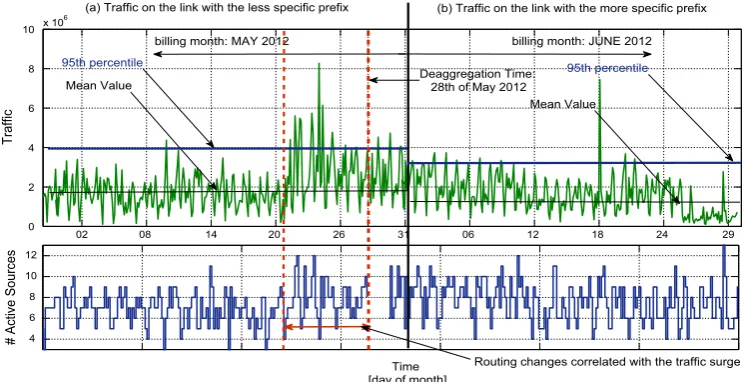
For the quantification of the impact of strategic deaggre-gation on the transit bill, we compare the traffic pattern for the identified prefix during a month prior to the moment of deaggregation (i.e. May) with the traffic pattern for the more-specific during a month after the moment of deaggre-gation (i.e. June). Since the billing period used by the Japanese ISP is the exact calendar month, we compare the bill from May with the bill from June. In order to extract from the traffic collection the data that interest us, we must first identify the physical links connecting the customer network under study and the provider. By parsing all the router con-figuration files, we obtain the identity of all the interfaces on the routers connecting the two networks. We then evaluate the chargeable amount of traffic for each case using the 95th percentile billing rule. We conclude that, even if the expect-ed amounts of traffic for the two prefixes are comparable, the transit bill is20% lowerfor the customer AS after selec-tively injecting the deaggregated prefix, as observed inFig. 8. The difference in the chargeable volume of traffic per month may be due to the surge we observe in the traffic pro-file depicted inFig. 8during the first analyzed month. In order to check that this increase is caused by routing changes that influence the way large sources send their traf-fic towards the destination AS, we would need a complete

view of the evolution in time of the BGP routing tables for the source networks. However, this type of information is unavailable at this point. Instead, we observe the changes in the number of active sources out of the top 20 which for-ward their traffic to the destination prefix via the Japanese provider, as depicted inFig. 8. We extract this information from the NetFlow traffic data of the Japanese ISP. The ana-lyzed sources are prefixes with length 24 and are responsible for more than 50% of the total traffic towards the destination prefix. After the injection of the more-specific prefix, the traffic has a more stable behavior than in the previous case and, also, the number of active traffic sources is more stable in time. We can also notice that there is a symmetry between the surge of traffic and an increase in the number of sources that forward their traffic through the transit link. The observed correlation between routing changes and traffic fluctuations supports the hypothesis according to which the 95th percentile billing rule can be gamed by the cus-tomer networks by restricting the choices of transit links diversity towards the destination prefix. However, we can-not demonstrate the causality between the changes we observe in the traffic pattern and the deaggregation strategy being deployed because of the lack of interest cases which fulfill the model requirements.

Based on the single perfect match for the strategic deag-gregation previously identified, we can only conclude that the study result supports the analytic observations for the economic impact of deaggregation.

7. Discussion

We proposed a novel methodology to identify all the cas-es of strategic deaggregation generated by the customers of any ISP and measure their economic side-effect. The methodology comes also with a number of limitations and challenges, which we hereafter explain and address.

In order to identify real occurrences of the interest sce-nario, we demonstrate the use of this methodology on the real data from an operational ISP. We obtain all the neces-sary information from a major Japanese ISP. This includes routing data that enable us to monitor how customers advertise their address space over time and the correspond-ing traffic traces, router configuration information needed to identify on which links to look for the traffic data and finally, the billing scheme used. The quality of the results is condi-tioned by the quality of the data. Though the amount of information we handle is very large, it does not offer perfect information regarding the operations of the customers.

The Japanese ISP maintains fine-grained traffic infor-mation for its customer prefixes only for the latest two months from the present moment of analysis. Consequently, the complete dataset from the major active ISP spans over a period of two months. Since we require the traffic traces both before and after the strategic deaggre-gation mechanism was deployed, this limits the traffic ana-lysis only to cases of strategic deaggregation that have occurred as far as one month previous to the moment of analysis.

We validate that the more-specific prefixes are selective-ly advertised onselective-ly towards the Japanese ISP using all the routing information gathered from ASes that are active in

Table 1

Number of deaggregating customer ASes and total advertised deaggregated prefixes per month.

Month No. of customer ASes No. of more-specifics

May 7 154

June 1 3

July 2 3

August 6 19

September 5 42

October 2 12

8

the RIPE RIS and RouteViews projects. Given that the num-ber of monitors active within the RIPE RIS and RouteViews project is limited to approximately 150, we have only a par-tial picture of how external sources of traffic reach the pre-fixes identified. Consequently, a prefix may be thought to be selectively advertised when it is in fact advertised to mul-tiple providers. In this case, though, we should not see a low-er transit bill than in the aggregated case.

When analyzing the real data from the Japanese ISP, we do not observe many cases of strategic deaggregation occur-ring within the time-window of interest. Though we do find a number of general deaggregation cases, the corresponding prefixes look like expressions of stable strategies, justified by general operational practices. Consequently, this does not allow for an extensive evaluation of the impact of this deaggregation strategy at the economic level.

All together, in the context of the Japanese Internet community we conclude that strategic deaggregation is generally not a practice used actively within the customer base. The results of our study show that the customers of the Japanese ISP do not make an extensive use of prefix deaggregation in general, and even less in the strategic form defined in this paper. There are a number of reasons why this may be the case, including the general pressure of the community regarding the negative impact of deaggre-gation, the unwillingness to increase the overall com-plexity of the Internet or even the lack of basic necessary expertise which would allow the deployment of such strategies at the interdomain level. It is, however, impor-tant to keep in mind that these conclusions are based on data from one major ISP, and the results may be different for