Real-Time Digital Signal Recovery for a Low-Pass Transfer Function System with Multiple Complex Poles

(1)

Article

Real-Time Digital Signal Recovery for a Low-Pass

Transfer Function System with Multiple Complex

Poles

Jhinhwan Lee

1,

*

1_{Department of Physics, Korea Advanced Institute of Science and Technology, Daejeon 34141, Korea}

* Correspondence: [email protected]; Tel.: +82-10-8584-6580

Abstract:

In order to solve the problems of waveform distortion and signal delay by many physical

and electrical systems with linear low-pass transfer characteristics with multiple complex poles, a

general digital-signal-processing (DSP)-based method of real-time recovery of the original source

waveform from the distorted output waveform is proposed. From the convolution kernel

representation of a multiple-pole low-pass transfer function with an arbitrary denominator

polynomial with real valued coefficients, it is shown that the source waveform can be accurately

recovered in real time using a particular moving average algorithm with real-valued DSP

computations only, even though some or all of the poles are complex. The proposed digital signal

recovery method is DC-accurate and unaffected by initial conditions, transient signals, and resonant

amplitude enhancement. This method can be applied to most sensors and amplifiers operating close

to their frequency response limits or around their resonance frequencies to accurately deconvolute

the multiple-pole characteristics and to improve the overall performances of data acquisition

systems and digital feedback control systems.

Keywords:

signal recovery; deconvolution; transfer function; digital signal processing

1. Introduction

Many sensors and amplifiers suffer from delayed and distorted responses with single- or

multi-pole low-pass characteristics when operated close to their frequency response limits or resonance

frequencies. Notable examples of multiple complex pole systems include a geophone sensor shown

in Fig. 1 and a piezoelectric accelerometer shown in Fig. 2. Unlike a first-order-response system, a

second or higher order system may have complex-conjugate-paired poles even though all the

coefficients of the denominator polynomial are real. This condition leads to resonant underdamped

transfer characteristics and requires a carefully thought-out digital signal recovery algorithm in a

conventional DSP system. Here I propose a real-time numerical waveform recovery method that is

suitable for the cases of arbitrary order multiple complex pole low pass transfer function systems and

discuss their detailed implementation method, accuracy and noise characteristics.

2. Mathematical analysis and development for linear systems with multiple complex poles

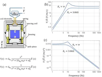
Let’s consider a two-pole low-pass system as shown in Fig. 1(a) which is a geophone sensor

optionally shunted with a resistor. With no or large shunt resistance, the damping parameter

𝛾

is

small and the denominator may have two complex conjugate poles leading to an underdamped

resonance behavior. This condition makes the previous method with real-valued poles [1] becomes

inappropriate due to the requirement of complex-valued calculations (i.e.

𝛾 = 𝑒

are complex for

complex

𝑠

) in the real-time core of the DSP/FPGA signal processor.

(2)

Figure 1. Geophone sensor with two-pole transfer functions with two complex conjugate poles. (a) Schematic diagram with a shunt resistor used for damping control, adopted from Ref 2, and its transfer functions. (b) The frequency characteristics of 𝑉(𝑠)/𝑋̇(𝑠) of a typical geophone for two

different 𝑅 values. (c) The frequency characteristics of 𝑉(𝑠)/𝑋(𝑠) for two different 𝑅 values.

Figure 2. Piezoelectric acceleration sensor with three-pole transfer functions with two complex conjugate poles and one real pole. (a) Schematic diagram adopted from Ref. 3 and its transfer functions. (b)-(c) The frequency characteristics of 𝑉(𝑠)/𝑋̈(𝑠) and 𝑉(𝑠)/𝑋(𝑠) of a typical

(3)

Here I will begin with an appropriate digital signal recovery method for a general two-pole

linear low-pass system by direct mathematical expansion starting from the convolution kernel

expression of the two pole transfer characteristics and show that it is equivalent to the nested

multi-pole solution shown in Fig. 4 of Ref. [1]. The results will then be generalized into higher order

low-pass system whose Laplace transfer function has an

n

-th order real-coefficient polynomial as its

denominator.

The Laplace representation of the first order low pass characteristics

with an initial condition

(Ref.

[4])

𝑉 (𝑠) =

/

𝑉 (𝑠) +

𝑉 (𝑡 = 0)

(1)

with time constant

𝜏 = 1/𝑠

can be converted to the time domain expression of

𝑉 (𝑡) = ∫ 𝑑𝑡 𝑠 𝑒

𝑉 (𝑡 − 𝑡′) + 𝑉 (𝑡 = 0)𝑒

Θ(𝑡)

.

(2)

We can recover the original signal as derived in Ref. [1]

𝑉 𝑡 −

≈

( ) ( )

(3)

since the contribution from the initial condition term

𝑉 (𝑡) = 𝑉 (𝑡 = 0)𝑒

Θ(𝑡)

vanishes as

( ) ( )

= 𝑉 (𝑡 = 0)

( ) ( ) ( )

= 0

(4)

for arbitrary

𝑡 > 𝑇

.

Now let’s consider the general second order low-pass characteristics with initial conditions

𝑉 (𝑠) =

𝑉 (𝑠) +

𝑉 (𝑡 = 0) +

𝑉′ (𝑡 = 0)

(5)

=

𝑉 (𝑠) +

𝑑 +

𝑑

.

(6)

This can be converted to the time domain solution of

𝑉 (𝑡) = 𝑉 (𝑡) + 𝑉 (𝑡)

(7)

which is the sum of the nested time domain convolution

𝑉 (𝑡) = ∫ 𝑑𝑡 𝑠 𝑒

∫ 𝑑𝑡 𝑠 𝑒

𝑉 (𝑡 − 𝑡 − 𝑡′′)

(8)

and the transient solution dependent on the initial conditions

𝑉 (𝑡) = 𝑑 𝑒

Θ(𝑡) + 𝑑 𝑒

Θ(𝑡)

.

(9)

Since

𝑉 (𝑡 − 𝑇) = ∫ 𝑑𝑡 𝑠 𝑒

𝑉 (𝑡 − 𝑇 − 𝑡 − 𝑡′′)

(10)

= 𝑒

𝑉 (𝑡 − 𝑡 − 𝑡′′)

(11)

(4)

and

𝑉 (𝑡 − 2𝑇) = 𝑒

𝑒

𝑉 (𝑡 − 𝑡 − 𝑡′′)

,

(13)

we have

𝑉 (𝑡 − 𝑡 − 𝑡′′) = 𝑉 (𝑡) − 𝑒

𝑉 (𝑡 − 𝑇) − 𝑒

𝑉 (𝑡 − 𝑇) +

𝑒

𝑉 (𝑡 − 2𝑇)

(14)

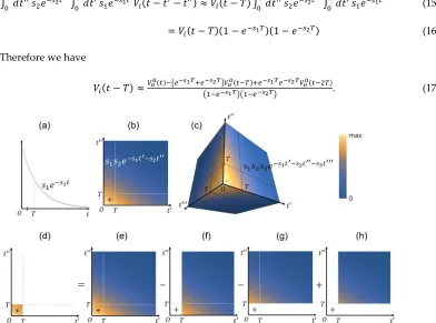
which is graphically illustrated in Fig. 3(d)-(h).

In the limit of small

𝑇

, the average value of

𝑉

over the square region of integration with

parameter range

[𝑡 − 2𝑇, 𝑡]

can be approximated by

𝑉 (𝑡 − 𝑇)

and the left-hand side expression is

simplified as

𝑉 (𝑡 − 𝑡 − 𝑡′′) ≈ 𝑉 (𝑡 − 𝑇) ∫ 𝑑𝑡 𝑠 𝑒

(15)

= 𝑉 (𝑡 − 𝑇)(1 − 𝑒

)(1 − 𝑒

)

(16)

Therefore we have

𝑉 (𝑡 − 𝑇) ≈

( ) ( ) ( )

.

(17)

Figure 3. (a)-(c) Convolution kernel functions for single-pole (𝑑 = 1) (a), two-pole (𝑑 = 2) (b) and

three-pole (𝑑 = 3) (c) low-pass systems. We assumed real values for 𝑠 , 𝑠 , 𝑠 , … for simplicity but

some of them can be complex conjugated pairs while unpaired ones should be real. The input function’s value at the center of the cubical volume 𝑇 can be well approximated by the convolution

integral within the cubical volume 𝑇 (that can be evaluated by subtracting and adding convolution

integrals with all possible combinations of time domain offsets as illustrated in (d)-(h) for 𝑑 = 2)

divided by the kernel-only integral within the same volume. The convolution integrals over the shaded regions in (d)-(h) are as follows.

(d) ∫ 𝑑𝑡 𝑠 𝑒 ∫ 𝑑𝑡 𝑠 𝑒 𝑉 (𝑡 − 𝑡 − 𝑡′′) ≈ 𝑽𝒊(𝒕 − 𝑻)(𝟏 − 𝒆 𝒔𝟏𝑻)(𝟏 − 𝒆 𝒔𝟐𝑻)

(e) ∫ 𝑑𝑡 𝑠 𝑒 ∫ 𝑑𝑡 𝑠 𝑒 𝑉 (𝑡 − 𝑡 − 𝑡′′) = 𝑽𝒐(𝒕)

(f) 𝑒 ∫ 𝑑𝑡 𝑠 𝑒 ∫ 𝑑𝑡 𝑠 𝑒 𝑉 (𝑡 − 𝑡 − 𝑡′′) = 𝒆 𝒔𝟏𝑻_𝑽_𝒐(𝒕 − 𝑻)

(g) 𝑒 ∫ 𝑑𝑡 𝑠 𝑒 ∫ 𝑑𝑡 𝑠 𝑒 𝑉 (𝑡 − 𝑡 − 𝑡′′) = 𝒆 𝒔𝟐𝑻_𝑽

𝒐(𝒕 − 𝑻)

(h) 𝑒 𝑒 ∫ 𝑑𝑡 𝑠 𝑒 ∫ 𝑑𝑡 𝑠 𝑒 𝑉 (𝑡 − 𝑡 − 𝑡′′) = 𝒆 𝒔𝟏𝑻_𝒆 𝒔𝟐𝑻_𝑽

(5)

Since for both

𝑖 = 1, 2

we have

𝑒

− {𝑒

+ 𝑒

}𝑒

( )

+ 𝑒

𝑒

( )

= 0

,

(18)

the contribution from the initial-condition-dependent transient solution

𝑉 (𝑡)

vanishes for arbitrary

𝑡 > 2𝑇

when inserted in the places of the

𝑉 (𝑡)

:

( ) ( ) ( )

= 0

.

(19)

Therefore the signal recovery formula for

𝑉 (𝑡)

maintains the same form as the Eq. (17):

𝑉 (𝑡 − 𝑇) ≈

( ) ( ) ( )

.

(20)

We can also show that the above Eq. (20) can be converted to a nested form

𝑉 (𝑡 − 𝑇) ≈

( ) ( ) ( ) ( )

(21)

=

( ) ( )

(22)

where we define the intermediately recovered waveform

𝑉 (𝑡) =

( ) ( )

.

(23)

This shows clearly that the single register implementation of the Eq. (20) is equivalent to the

cascaded two register implementation shown in Fig. 4 of Ref. [1].

The above result can be generalized to an arbitrary high order

𝑛

. The general

𝑛

-th order

low-pass characteristics with initial conditions is given by

𝑉 (𝑠) =

∑

𝑉 (𝑠) +

∑ ∑ ( )( )

∑

(24)

=

∏

𝑉 (𝑠) + ∑

𝑑

(25)

where

𝑑

is a linear combination of the initial conditions

𝑉

( , , ,…, )

(𝑡 = 0)

[4].

The time-domain solution is given in the form

𝑉 (𝑡) = 𝑉 (𝑡) + 𝑉 (𝑡)

(26)

where

𝑉 (𝑡) = ∫ 𝑑𝑡 𝑠 𝑒

⋯ ∫ 𝑑𝑡 𝑠 𝑒

𝑉 (𝑡 − 𝑡 − 𝑡 − ⋯ − 𝑡 )

(27)

and

𝑉 (𝑡) = ∑

𝑑 𝑒

Θ(𝑡)

.

(28)

(6)

𝑉 𝑡 − 𝑛 ≈

( ) ⋯ ( ) ⋯ ( ) ⋯ ( ) ⋯ ( )

⋯

(29)

where the coefficients for

𝑉 (𝑡 − 𝑚𝑇)

in the numerator are simply the coefficients for the

𝑧

term

in the generating polynomial

𝐹(𝑧) = (𝑧 − 𝑒

)(𝑧 − 𝑒

) ⋯ (𝑧 − 𝑒

)

.

(30)

We can again show that the transient solution

𝑉 (𝑡)

gives no contribution to the right-hand side

of the Eq. (29) since, for the arbitrary

𝑖

-th term of the Eq. (28) proportional to

𝑒

, we have

𝑒

− {𝑒

+ 𝑒

+ ⋯ + 𝑒

}𝑒

( )

+ {𝑒

𝑒

+ 𝑒

𝑒

+ ⋯ + 𝑒

𝑒

}𝑒

( )

+ ⋯ + (−1) {𝑒

𝑒

⋯ 𝑒

}𝑒

( )

= 𝑒

( )

⎣

⎢

⎡

𝑒

−{𝑒

+ 𝑒

+ ⋯ + 𝑒

}𝑒

( )

+{𝑒

𝑒

+ 𝑒

𝑒

+ ⋯ + 𝑒

𝑒

}𝑒

( )

+ ⋯

+(−1) {𝑒

𝑒

⋯ 𝑒

}

⎦

⎥

⎤

(31)

= 𝑒

( )

𝐹(𝑒

) = 0

(32)

and the right-hand side of the Eq. (29) vanishes when

𝑉 (𝑡)

is replaced by

𝑉 (𝑡)

.

This provides a general proof that the signal recovery method shown in the Eq. (29) produces

output signal completely independent of the initial conditions and the transient signals.

3. Real-valued device implementation

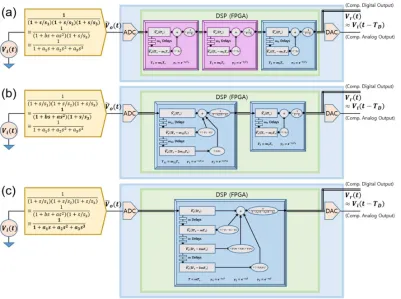
Fig. 4 shows three equivalent representations for physical implementation of high order signal

recovery in the DSP/FPGA device. They are mathematically equivalent but in case of complex poles,

the first implementation (Fig. 4(a)) requires complex computation while the second (Fig. 4(b)) and

the third (Fig. 4(c)) require only real-valued computation which has a significant advantage in the

real-time process core of the DSP/FPGA.

We note that the complex roots of any real-coefficient polynomial always occur in

complex-conjugated pairs. Therefore in the device implementation of Fig. 4(b) (formed by combining every

pair of register loops of Fig. 4a for a complex conjugate pair (such as

𝑠

and

𝑠

with

𝐷 = 𝑏 − 4𝑎 <

0

) into a single register loop), it is sufficient to show that only real-valued computations are needed

for the evaluation of the combined second order Eq. (20).

Let’s assume that

𝑠 = 𝛼 + 𝑖𝛽

and

𝑠 = 𝛼 − 𝑖𝛽

where

𝛼

and

𝛽

are real and

𝛼 > 0

. Then we

have the following values all real:

𝑒

+ 𝑒

= 𝑒

( )

+ 𝑒

( )

= 2𝑒

cos 𝛽𝑇

(33)

𝑒

= 𝑒

( ) ( )

= 𝑒

(34)

(7)

𝑉 (𝑡 − 𝑇) ≈

( ) ( ) ( )

.

(35)

The device implementation of Fig. 4(c) (formed by combining all the register loops of Fig. 4a into

one) also has the property of real-value-only computations. The proof that all the coefficients in the

numerator of the Eq. (29) and its denominator are real-valued is easily provided noting that if

𝑠

and

𝑠

are a complex-conjugate pair,

𝑒

and

𝑒

are also. As a result, all the coefficients of the

polynomial expansion of the Eq. (30) are real. Therefore, all the coefficients appearing in the

numerator of Eq. (29) are real and the denominator

𝐹(1)

is real.

4. Noise consideration

In order to understand the noise characteristics of the multi-pole recovery method

quantitatively, let’s assume without too much loss of generality, that the high-order-convoluted

analog output signal

𝑉 (𝑡)

contains a slow-varying (compared to

2𝑇

) raw signal

𝑉 (𝑡)

plus a

pseudo-random noise

𝑉 (𝑡)

whose correlation time is shorter than

𝑇

. First, let’s look at the

nontrivial second-order case of Eq. (35) where the two roots

𝑠

and

𝑠

are a complex-conjugated

pair.

Figure 4. Schematic diagrams of a real-time digital signal recovery system compensating for the signal distortion by a physical or electrical system with multi-pole low-pass transfer characteristics (in yellow pentagons on the left). (a) In case all the 𝑠 are real and positive, the nested multiple register

scheme as illustrated in Ref. [1] can be used. However, in case some of the 𝑠 are complex, the scheme

is not efficiently realized in real-valued digital signal processors. For example, if 𝑠 and 𝑠 are

complex conjugates and 𝑠 is real, the processes in the purple boxes requires complex-valued

calculations. Two alternative solutions are suggested: (b) Combining two registers for every complex conjugated pair of the 𝑠 (e.g. 𝐷 = 𝑏 − 4𝑎 < 0) into one, while leaving the registers for real 𝑠 left

(8)

Then the numerical recovery operation applied to

𝑉 (𝑡) = 𝑉 (𝑡) + 𝑉 (𝑡)

can be divided into two

terms

𝑉 (𝑡 − 𝑇) ≈

( ) ( ) ( )

+

( ) ( ) ( )

(36)

where the first term gives the slow varying signal with value approximated by

𝑉 (𝑡)(≈

𝑉 (𝑡 − 𝑇) ≈ 𝑉 (𝑡 − 2𝑇))

and the second term gives noise level proportional to

( )

|

𝑉

_𝑛

(𝑡)

|

due to the presumed absence of time correlation between noise

𝑉 (𝑡)

,

𝑉 (𝑡 − 𝑇)

, and

𝑉 (𝑡 − 2𝑇)

. For small

𝛼𝑇 ≪ 1

and

𝛽𝑇 ≪ 1

, the signal-to-noise (S/N) ratio is

reduced by a factor of

≈

1−2𝑒−𝛼𝑇cos 𝛽𝑇+𝑒−2𝛼𝑇

1+ 2𝑒−𝛼𝑇_{cos 𝛽𝑇}2_+𝑒−4𝛼𝑇

≈

𝛼

2_+𝛽2 _𝑇2

6

=

√

≪ 1

.

(37)

This is formally identical to the result when the two poles are real

≈

√

.

(38)

Generalization to an arbitrarily high order case of Eq. (29) leads to

≈

⋯

⋯ ⋯ ⋯ ⋯

(39)

≈

| ⋯ |

_{⋯ {} _}

(40)

=

| ⋯ |

.

(41)

As mentioned in Ref. [1], if we sample

𝑉 (𝑡)

𝑁 (≥ 2)

times over the short time intervals within

[𝑡, 𝑡 − 𝑇)

and use their averages in place of

𝑉 (𝑡)

, we may further increase the S/N by up to a factor

given by a fraction of

𝑁

. The factor can approach

𝑁

in case the correlation time of the noise is

still shorter than the sampling periods of the

𝑁

data points. On the other hand, when it is possible

to perform

𝑁

multiple measurements over a repeated input signal, we can increase the S/N to an

arbitrary level by choosing the averaging

𝑁

by

𝑁 ≥

| ⋯ |

(42)

5. Simulated demonstrations

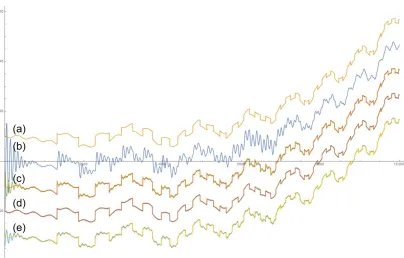
I performed simulations for an underdamped two-pole geophone sensor system shown in Fig.

1 and a three-pole piezoelectric accelerometer shown in Fig. 2 whose results are shown in Figs. 5-7

and Figs. 8-10 respectively. We first numerically solved the second order differential equations for

three different kinds of input waveforms and processed it with the real-time data recovery scheme

shown in Fig. 3(c) with an optimal and two non-optimal choices of parameters.

As can be seen in all Figs. 5-10, the recovered waveform closely matches with the input

waveform only when the parameter

𝑇

used in evaluating all the coefficients of the Eq. (20) or (29)

(9)

coefficients and hence the optimal overall compensation. Also it should be noted that the signal

recovery is DC-accurate and independent of the initial conditions, the transient waveforms and the

waveforms significantly amplified near the resonance frequency.

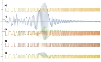
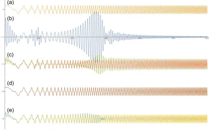
Figure 5. Numerical simulation of the real-time waveform recovery in the scheme of Fig. 4(c) for a system with two-pole transfer characteristics shown in Fig. 1(a), tested with a frequency-varying rectangular input waveform. (a) Input waveform 𝑉 (𝑡) ≡ 𝐺 𝑋(𝑡). (b) Response of the system output 𝑉 (𝑡) calculated by numerically solving the differential equation with the two initial conditions 𝑉 (0)

and 𝑉̇ (0) arbitrarily chosen. (c) Compensated waveform 𝑉 (𝑡) (overlaid with the input waveform 𝑉 (𝑡)) calculated from the waveform in (b) with all the 𝛾 parameters intentionally offset from their

optimal values by replacing every 𝑇 by 0.9𝑇. (d) Compensated waveform 𝑉 (𝑡) (overlaid with the

input waveform 𝑉 (𝑡)) calculated from the waveform in (b) with all the 𝛾 parameters set at their

optimal values. (e) Compensated waveform 𝑉 (𝑡) (overlaid with the input waveform 𝑉 (𝑡))

calculated from the waveform in (b) with all the 𝛾 parameters intentionally offset from their optimal

values by replacing every 𝑇 by 1.1𝑇. Note that the strong transient waveforms after the sharp

transitions and the strong resonant waveform near 2000 < 𝑡 < 3500 in (b) are exactly cancelled out

(10)

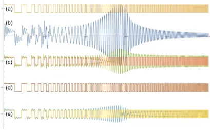
Figure 6. Numerical simulation of the real-time waveform recovery in the scheme of Fig. 4(c) for a system with two-pole transfer characteristics shown in Fig. 1(a), tested with a frequency-varying cosine-cubed input waveform. (a) Input waveform 𝑉 (𝑡) ≡ 𝐺 𝑋(𝑡). (b) Response of the system

output 𝑉 (𝑡) calculated by numerically solving the differential equation with the two initial

conditions 𝑉 (0) and 𝑉̇ (0) arbitrarily chosen. (c) Compensated waveform 𝑉 (𝑡) (overlaid with the

input waveform 𝑉 (𝑡)) calculated from the waveform in (b) with all the 𝛾 parameters intentionally

offset from their optimal values by replacing every 𝑇 by 0.9𝑇. (d) Compensated waveform 𝑉 (𝑡)

(overlaid with the input waveform 𝑉 (𝑡)) calculated from the waveform in (b) with all the 𝛾

parameters set at their optimal values. (e) Compensated waveform 𝑉 (𝑡) (overlaid with the input

waveform 𝑉 (𝑡)) calculated from the waveform in (b) with all the 𝛾 parameters intentionally offset

from their optimal values by replacing every 𝑇 by 1.1𝑇. Note that the strong transient waveform

near 0 < 𝑡 < 400 in (b) and the strong resonant waveform near 2000 < 𝑡 < 3500 are exactly

(11)

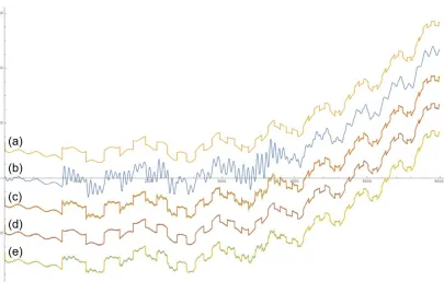
Figure 7. Numerical simulation of the real-time waveform recovery in the scheme of Fig. 4(c) for a system with two-pole transfer characteristics shown in Fig. 1(a), tested with an aperiodic input waveform. (a) Input waveform 𝑉 (𝑡) ≡ 𝐺 𝑋(𝑡). (b) Response of the system output 𝑉 (𝑡) calculated

by numerically solving the differential equation with the two initial conditions 𝑉 (0) and 𝑉̇ (0)

arbitrarily chosen. (c) Compensated waveform 𝑉 (𝑡) (overlaid with the input waveform 𝑉 (𝑡))

values by replacing every 𝑇 by 0.9𝑇. (d) Compensated waveform 𝑉 (𝑡) (overlaid with the input

waveform 𝑉 (𝑡)) calculated from the waveform in (b) with all the 𝛾 parameters set at their optimal

values. (e) Compensated waveform 𝑉 (𝑡) (overlaid with the input waveform 𝑉 (𝑡)) calculated from

the waveform in (b) with all the 𝛾 parameters intentionally offset from their optimal values by

replacing every 𝑇 by 1.1𝑇. Note that the strong transient waveforms after the sharp transitions are

(12)

Figure 8. Numerical simulation of the real-time waveform recovery in the scheme of Fig. 4(c) for a system with three-pole transfer characteristics shown in Fig. 2(a), tested with a frequency-varying rectangular input waveform. (a) Input waveform 𝑉 (𝑡) ≡ 𝐺𝜔 𝑋(𝑡). (b) Response of the system output 𝑉 (𝑡) calculated by numerically solving the differential equation with the two initial conditions 𝑉 (0)

and 𝑉̇ (0) arbitrarily chosen. (c) Compensated waveform 𝑉 (𝑡) (overlaid with the input waveform 𝑉 (𝑡)) calculated from the waveform in (b) with all the 𝛾 parameters intentionally offset from their

optimal values by replacing every 𝑇 by 0.9𝑇. (d) Compensated waveform 𝑉 (𝑡) (overlaid with the

input waveform 𝑉 (𝑡)) calculated from the waveform in (b) with all the 𝛾 parameters set at their

optimal values. (e) Compensated waveform 𝑉 (𝑡) (overlaid with the input waveform 𝑉 (𝑡))

values by replacing every 𝑇 by 1.1𝑇. Note that the strong transient waveforms after the sharp

(13)

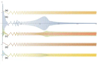
Figure 9. Numerical simulation of the real-time waveform recovery in the scheme of Fig. 4(c) for a system with three-pole transfer characteristics shown in Fig. 2(a), tested with a frequency-varying cosine-cubed input waveform. (a) Input waveform 𝑉 (𝑡) ≡ 𝐺𝜔 𝑋(𝑡). (b) Response of the system

References

1. Jhinhwan Lee, "Real-time digital signal recovery for a multi-pole low-pass transfer function system", Review of Scientific Instruments 88, 085104 (2017)
2. M. Kamata, “High Precision Geophone Calibration”, J. Acoustic Emission, 23, 81 (2005)
3. “Piezoelectric Accelerometers, Theory and Application”, Metra Mess-und Frequenztechnik (2001)
4. Hazewinkel, Michiel, ed., "Laplace transform" in Encyclopedia of Mathematics, Springer, 2001
5. Alan V. Oppenheim and Ronald W. Schafer, “Ceptrum Analysis and Homomorphic Deconvolution”
in Discrete-Time Signal Processing, Englewood Cliffs, NJ, USA: Prentice Hall, 1989
6. Steven W. Smith, “Custom Filters” in The Scientist and Engineer's Guide to Digital Signal Processing, 1st ed. San Diego, CA, USA: California Technical Publishing, 1997
7. D. S.G. Pollock, Richard C. Green and Truong Nguyen, "Linear Filters" in Handbook of Time Series Analysis, Signal Processing, and Dynamics, Elsevier, 1999
8. B. Widrow and S.D. Stearns, Adaptive Signal Processing, Pearson, 1985
9. D.G.Manolakis, V.K. Ingle and S.M.Kogon, Statistical and Adaptive Signal Processing, McGraw Hill, 2005
10. E. Ifeachor and B. Jervis, Digital Signal Processing: A Practical Approach, 2nd ed. Prentice Hall, 2002