Article
Multi-range Conditional Random Field for
Classifying Railway Electrification System Objects
Jaewook Jung 1,†, Leihan Chen 1,†, Gunho Sohn 1,*, Chao Luo 1 and Jong-Un Won 2
1 Department of Earth and Space Science and Engineering, York University, 4700 Keele Street, Toronto, ON M3J 1P3, Canada; [email protected] (J.J); [email protected] (L.C.) ; [email protected] (C.L.) ;
2 Logistics System Research Team, Korea Railroad Research Institute, 176, Cheoldobangmulgwan-ro, Uiwang-si 437-757, Gyeonggi-do, South Korea ; [email protected] (J.-U.W.) ;
* Correspondence: [email protected] ; Tel.: +1-416-650-8011;
† The co-first author Dr. Jung and Mr. Chen have equal contribution to this manuscript as co-first authors.
Abstract: Railway has been used as one of the most crucial means of transportation in public mobility and economic development. For efficiently operating railways, the electrification system in railway infrastructure, which supplies electric power to trains, is essential facilities for stable train operation. Due to its important role, the electrification system needs to be rigorously and regularly inspected and managed. This paper presents a supervised learning method to classify Mobile Laser Scanning (MLS) data into ten target classes representing overhead wires, movable brackets and poles, which are recognized key objects in the electrification system. In general, the layout of railway electrification system shows a strong regularity of spatial relations among object classes. The proposed classifier is developed based on Conditional Random Field (CRF), which characterizes not only labeling homogeneity at short range, but also the layout compatibility between different object classes at long range in the probabilistic graphical model. This multi-range CRF model consists of a unary term and three pairwise contextual terms. In order to gain computational efficiency, MLS point clouds is converted into a set of line segments where the labeling process is applied. Support Vector Machine (SVM) is used as a local classifier considering only node features for producing the unary potentials of CRF model. As the short-range pairwise contextual term, Potts model is applied to enforce a local smoothness in short-range graph. While, long-range pairwise potentials are designed to enhance spatial regularities of both horizontal and vertical layouts among railway objects. We formulate two long-range pairwise potentials as the log posterior probability obtained by Naïve Bayes classifier. The directional layout compatibilities are characterized in probability look-up tables which represent co-occurrence rate of spatial relations in horizontal and vertical directions. The likelihood function is formulated by multivariate Gaussian distributions. In the proposed multi-range CRF model, the weight parameters to balance four sub-terms are estimated by applying the Stochastic Gradient Descent (SGD). The results show that the proposed multi-range CRF can effectively classify detailed railway elements, representing the average recall of 97.66% and the average precision of 97.07% for all classes.
Keywords: classification; railway; power line; mobile laser scanning data; conditional random field; layout compatibility
1. Introduction
electrification system supplies a power that the train can access at all times. It must be safe, reliable, economical and user friendly. Therefore, rigorous inspection and frequent maintenance of railway electrification system are essential and regular tasks. However, the railway infrastructure is still vulnerable to a number of potential risks such as structural defects, equipment failure, vegetation encroachment, severe weather conditions, human factors and so forth [2]. To timely mitigate such risks, today’s inspection practice mainly relies on labor intensive visual inspection by human’s traversing along the rail tracks. However, this traditional monitoring of rail electrification systems is tedious, time-consuming and inaccurate [4].
Recently, various techniques using remotely sensed data such as images, airborne laser scanning (ALS) data and mobile laser scanning (MLS) data have been introduced to supplement or replace human’s visual inspection. In particular, MLS data provides very accurate and highly dense point clouds over railway scene by scanning laser scanners mounted on a train or inspection cart. In many previous researches, MLS data has been used to automatically recognize, detect, and reconstruct specific elements of railway infrastructure such as rails, power lines, and poles. For instance, Jwa and Sohn [5] and Arastounia [2] recently reported their success to automatically detect key elements of railway corridor infrastructure from MLS data in limited environments. However, fully understanding or analysis of railway scene is not an easy task because railway infrastructure consists of various elements such as tracks, poles, wires, equipment, traffic signs, tunnels and stations which complicate scene analysis. Moreover, even same objects have different types according to their functions and in different regions. For instance, wires can be sub-categorized into electricity feeder, catenary wire, contact wire, current return wire, dropper and so forth. These complex elements make scene interpretation more challenging.
A first critical step for effective analysis of complex railway infrastructure from MLS data is to classify point clouds into meaningful railway objects. A supervised learning is one of the most popular classification methods, which identify a set of object categories from unknown observation on the basis of a training data. The training data used in the supervised classification contributes to either modeling of representative feature distribution characterizing individual object classes (generative learning) or determination of decision boundaries among object categories (discriminative learning). A typical supervised approach is to use a local classifier such as Support Vector Machine (SVM) which differentiate the object from the others mainly by representing local characteristics of apparent features. Even though the local classifiers can provide promising results, the methods do not consider the relations with neighbor objects. Thus, the local classifiers often lead to inhomogeneous results in complex scene [6]. Also, the misclassifications of local classifiers occur due to ambiguity in appearance feature, varying vision conditions and overlap of multiple classes in feature space [7]. These limitations of local classifiers can be supplemented by integrating context information between objects. This is based on the fact that adjacent objects are more likely to have same label, emphasizing local smoothness. The idea can be extended by layout compatibility of objects which are often observed in the scene. These relations can be designed in an integrated Conditional Random Field (CRF) model. In this regard, Luo and Sohn [7] proposed multi-range CRF which considers vertical and horizontal layout relations to improve local classification results.
Fortunately, even though railway infrastructure consists of complex objects, it has strong spatial regularities between railway elements. For instance, rail tracks have two linear objects which orthogonal distance is almost fixed; contact wire is just above center of rail with a certain height; catenary wire is also above contact wire; dropper connects between catenary wire and contact wire; current return wire and pole are located outside rails. These layout compatibility of railway elements can be explained by horizontal and/or vertical relations which can be used as a prior knowledge for classification of railway scene and considered in CRF model, reducing the ambiguities for scene analysis.
as unary potential of CRF model. Two different graphs are designed to consider local smoothness and long-range layout compatibilities in horizontal and vertical directions. The final classifier integrates both local smoothness and layout compatibilities in vertical and horizontal directions to incorporate as much contextual information as possible to improve the classification result of complex railway scene.
Related Works
Recently, due to the importance of inspection and management in railway infrastructure, many research works have been studied to interpret railway scene using remotely sensed data. The research works mainly focus on detecting and modeling specific railway objects such as wires, and rail tracks which are considered important objects. Zhang et al. [4] extracted power lines from MLS data, which are parallel to rail tracks using an adaptive region growing method. The extracted power lines points were modeled by fitting the points to a polynomial model. Muhamad et al. [8] proposed an automatic rail extraction method using terrestrial laser points and ALS data. In their work, railway tracks were modeled as a dynamic system of local pairs of parallel line segments. Kalman filter was used to predict and monitor the state of the system. A similar approach was applied by Jwa and Sohn [5] to detect and model rail tracks using MLS data. These research works mentioned above require well classified points which belong to objects to be modeled. In the previous researches, they extracted the points by considering specific properties of target object (e.g., height difference from ground) and did not classify entire scene. Although the methods may be useful to detect and model specific objects, classification for whole scene is required as prerequisite process to fully understand railway scene. In this regard, Kim and Sohn [9] proposed a point-based supervised classification method using ALS data. Random Forest (RF) was applied to identify five utility corridor objects (vegetation, wire, pylon, building, and low object). Guo et al. [10] proposed power line reconstruction method based on RANdom Sample Consensus (RANSAC) rule. Before reconstruction of power lines, ALS data was classified into five categories (power line, vegetation, building, ground and pylon) by applying JointBoost classifier. Even though their classification results showed promising results, a classification method for identifying more detailed objects is required to represent complex railway scene. Arastounia [2] proposed an automatic classification method to recognize railroad infrastructure from MLS data. In the paper, detailed objects such as rail tracks, contact wire, catenary wire, current return wire, masts and cantilevers were defined as key components of the railroad infrastructure. The key components were recognized by considering their physical shape, geometrical properties and the topological relationships among them with user-defined thresholds. Thus, a classification method, which can effectively identify detailed objects of railway infrastructure, needs to be proposed for further applications.
Traditionally, local classifiers such as Logistic Regression, SVM and RF have been widely used to classify objects in various environments. In terms of application using laser points data, Chehata et al. [11] applied RF for urban scene classification using full-waveform ALS data. Their results showed that approximately 94% overall accuracy was achieved by RF in urban area. Zhang et al. [12] applied segment-based SVM classifier to classify urban area. However, the main limitation of local classifiers is that they do not consider neighbor relations, causing ambiguities of features among classes. Thus, misclassifications are mainly occurred if objects have similar feature properties.
RF confidence was used as unary potential while pairwise potential encoded the dependency of a node from its adjacent node by comparing both node labels and considering the observed data. Similar approach was proposed by Nowozin et al. [15] to combine RF and CRF. Lim and Suter [16] segmented terrestrial laser data into adaptive support regions (super-voxel) and applied multi-scale CRF, which provides connectivity at local edges and regional levels, for super-voxel labeling.
Spatial layout is a kind of space configurations to show relative location among objects. Winn and Shotton [17] introduced a layout consistent random field (LayoutCRF) to formulate layout by applying asymmetric pairwise potential in their graphical model. Long-range spatial constraints were propagated via only local pairwise potential. Gould et al. [18] used relative location probability map to encode all relative locations observed from the training data by calculating co-occurrence rate. The co-occurrence rate showed how possible two objects follow a specific relative location. Even though the spatial layout was applied for image classification, there is few study on incorporating layout contextual information into point clouds classification. Luo and Sohn [7] applied multi-range asymmetric CRF for building facade classification using terrestrial laser scanning data. In their work, layout information is learned from a prior table which represents layout information obtained from training data. A multivariate Gaussian distribution was assumed to represent pairwise term. However, their CRF model was constructed at each profile and this causes limited contextual range for more sophisticated interaction between different objects. Our method extends the idea of this multi-range asymmetric CRF and apply it into the classification of challenging railway scene using high-density large scale MLS data.
The paper is organized as follows. Section 2 presents our integrated CRF model, its sub-terms and graph construction. Section 3 introduces training and inference of the proposed CRF model while Section 4 shows the experiment result. The paper concludes with Section 5.
2. Methods
The proposed multi-range classification method aims to classify important elements in railway infrastructure. Rail vectors, which were extracted using a method proposed by Jwa and Sohn [5], and MLS data are used as input data. Line-based classification is applied where linear segments are used as unit entity. After generating voxel structure from MLS data, linear segments for each voxel are extracted by applying RANSAC algorithm where points are considered as consensus if the distance between the point and a candidate line is smaller than a certain user-defined distance. Note that multiple linear segments can be extracted in each voxel. After applying SVM classifier, the proposed multi-range CRF, which consider short-range, horizontal long-range and vertical long-range relations, is applied to classify linear segments. In multi-range CRF, two different graphs, which represent short-range and long-range relations, respectively, are generated to define adjacent relationships. Based on generated graphs, integrated CRF is conducted to refine SVM results. Section 2.1 explains the proposed graphical model and combination strategy of sub-terms and Section 2.2 presents graph definition. Following sections introduce each sub-term of multi-range CRF.
2.1. Graphical Model Design
CRF is used to encode known relations between observations and to construct consistent interpretations. It usually consists of unary term, which represents the importance of each node, and pairwise term, which represents contextual information with a graph. In this paper, the contextual information is expressed by the local smoothness with a short-range graph and spatial layouts in both vertical and horizontal directions with a long-range graph. Thus, the proposed multi-range CRF consists of a combination of a unary term and three different pairwise terms. Unary term is designed to encode the likelihood of each node to be assigned with each label given the node features. Three pairwise terms formulate the local smoothness, vertical spatial layout and horizontal spatial layout through edges in the graphs given the observation of edge feature X.
( | ) = 1
( ) ( , ) , ,
∈
∈ (1)
where ( , ) is the unary potential and , , represents the pairwise potential. ( ) is
the normalization constant (partition function) to ensure the probability p sums up to 1. S is a set of nodes in the graph and represents the neighbors of node i connected via edges in the graph. Due to the monotonic property of logarithm, the Eq. (1) can also be expressed as follows:
( | ) = 1
( ) ( , )
∈
+ , ,
∈
(2)
where and is the weight parameters to balance the unary term and pairwise term, respectively. In our model, pairwise term in Eq. (2) is expanded to three pairwise terms as follows:
( | ) = 1
( ) ( , )
∈
+ , ,
∈
+ , ,
∈
+ , ,
∈
(3)
where ( , ), , , , , , and , , represent the unary potential,
short-range pairwise potential, vertical long-short-range pairwise potential and horizontal long-short-range pairwise potential, respectively. , , and are weight parameters for four sub-term, respectively.
2.2. Definition of the Graph
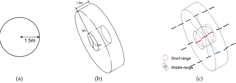
In a CRF model, dependent relations between nodes are defined by an adjacent graph. In image space, the adjacent relation is normally determined by adjacent pixels using standard four-connected neighborhood [19, 20] or using eight-connected neighborhood [21]. However, in laser scanning points which are irregularly distributed, the definition of adjacent relations is not straightforward. In previous researches using points data, neighborhood relations are defined by Delaunay Triangulation (DT) [22], k nearest neighbors [6] and super-voxels [16]. In our study, we need to define two different neighboring systems for establishing short-range relation and long-range relation. A sphere with a user-defined radius (1.5m in this paper) is used to define short-range relation (Figure 1(a)) while cylinder with hole is used for long-range relation (Figure 1(b)). The height and radius of the cylinder and the radius of hole are set as 5m, 1.5m and 1.5m, respectively. The orientation of the cylinder is determined by rail vector.
(a) (b) (c)
Once two types of neighboring systems are defined, graphs for short-range and long-range are generated. In graphs = ( , ), a node ( ∈ ) represents a line segment extracted from MLS data and node adjacent relation ∈ is constructed if a line is found in each neighboring system. As mentioned above, two different graphs, short-range graph and long-range graph, are generated for the proposed CRF model (G = G , G ). In short-range graph = ( , ), a line is considered as a neighbor node if the center point of the line is found in the sphere generated from other line. Note that an edge is excluded if the angle difference between two lines is significantly different with a user-defined threshold (30º in this paper). It is due to the fact that two lines, which have a larger angle difference, are likely to belong to different classes. Long-range graph = ( , ) is generated by applying cylinder with hole so that short-range relations are excluded. Also, a line whose center is below corresponding rail vector is excluded from long-range graph. It can largely reduce the number of long-range edges so that inference speed can be significantly accelerated. In both graphs, multiple edges for one line can be generated.
2.3 Unary Term
Unary term in Eq. (3) corresponds a log posterior probability of any label given observation . Because unary term only considers node features, the posterior probability of any local classifiers can be used. SVM is a very typical discriminative classifier which maps the data into a high-dimensional feature space and finds a hyperplane that separates feature space with the maximum margin [23]. SVM classifier shows a success in multiple-class classification problems. Thus, we firstly apply SVM classifier to classify our railway scene. In our SVM setting, we use six-dimensional features to represent the property of a line segment as follows:
• Point density: the density of points which support a line segment.
• Residuals: the standard deviation calculated from the line segment and its supporting points.
• Verticality: the vertical angle of the line.
• Horizontal angle: the angle between line segment and its corresponding rail vector in XY plane.
• Height: a height difference between a line segment and its corresponding railway vector.
• Distance: a horizontal distance between a line segment and its corresponding railway vector.
The SVM log posterior probability results are used as the unary term in our CRF model as follows:
( , ) = ( | ) (4)
2.4. Short-range Binary Term
The second term in Eq. (3) represents short-range pairwise term which is designed to enforce local smoothness. Local smoothness is a universal assumption that things in the physical world are spatial smooth [24], which means that the neighbors of a line segment are more likely to have the same label than different labels. This term is designed by a Potts model favoring neighboring entities
i and j to have same label and penalizing the configuration of different labels. A Potts model is simple but quite effective to many smoothness applications. In our research, the short-range pairwise
potential , , can be expressed as follows:
= , = , = 1,0, =≠ (5)
2.5 Long-range Binary Term
attracts more attention in representing spatial layout. It can reflect relative locations for all objects in a map and then the map intensity represents how possible two objects co-occur in a certain pattern. For our long-range terms, we adopt the co-occurrence statistic to define “above-below” and “near-far” relations in both vertical and horizontal directions which are described in Section 2.5.1 and Section 2.5.2, respectively.
2.5.1 CRF based on Vertical Layout Compatibility
In order to embed vertical layout compatibility in CRF model, “above-below” relationship is modeled for long-range neighbors. Bayes rule is used to calculate posterior probability as follows:
= , = |
= | = , = ( = , = )
∑ ∈ , ∈ | = , = ( = , = )
(6)
where , is a pair of lines consisting of the edge in graph . indicates the node
above the other in the edge , while indicates the node below the other.
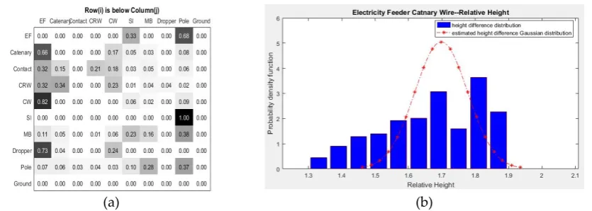
( = , = ) is the prior probability that class type is above class type . The prior probability is represented by the co-occurrence rate which is statistically obtained from training data. In this paper, the co-occurrence rate is formulated from a look-up table as shown in Figure 2(a). The likelihood function in Eq. (6) is the probability distribution function of edge given a configuration of that class is above class k, which quantitatively measures how class l can be found above class k. Here we use three-dimensional feature vector to represent edge . The feature vector consists of height difference, horizontal angle difference and verticality difference between two line segments. We make the assumption that the edge feature distribution follows a multivariate Gaussian distribution as follows:
= , = =
−12 − , Σ, − ,
2 Σ,
(7)
where , and Σ, are the mean vector and covariance matrix, respectively. In our study, the parameters are trained from the training data through Maximum Likelihood (ML) algorithm. Figure 2(b) shows the estimated probability distribution of height difference between electricity feeder and catenary wires. In the figure, the estimated probability distribution from training data fits the test data feature distribution well. It indicates that multivariate Gaussian distribution is applicable to the railway scene. Then, the vertical long-range pairwise term can be expressed as follows:
, , = = , = | (8)
With ten classes, which are introduced in Section 4.1, one hundred types of pairwise potentials are learned from the training data, generating different multivariate Gaussian distributions. The designed long-range potentials are not asymmetric because both our prior and likelihood are
asymmetric, which makes potential , , ≠ , , . This configuration will encourage
(a) (b)
Figure 2. Prior and likelihood estimation of vertical long-range pairwise potential; (a) Look-up table where row i is below column j and (b) probability density distribution of height difference (red curve: estimated Gaussian distribution learned from training data).
2.5.2 CRF based on horizontal Layout Compatibility
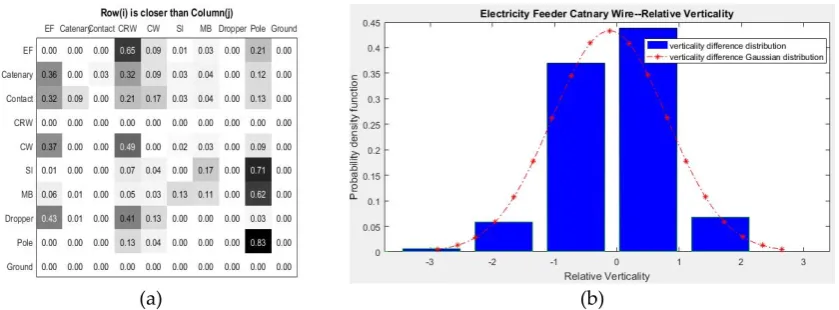
Similar to vertical long-range pairwise term, we model “near-far” relationship in this long-range horizontal pairwise term. The same long-range graph is used but different feature property is applied to represent near-far relationship. Three-dimensional feature vector which consists of horizontal angle difference, vertical angle difference, and horizontal distance difference, is formulated between two line segments. Bayes rule is also used to calculate posterior probability as follows:
= , = | = | = , = = , =
∑ ∈ , ∈ | = , = = , = (9)
where , is a pair of lines consisting of the edge in graph . and represent
horizontal relations between nodes.
In Eq. (6), = , = is the prior probability that class type is more near to railway
than class type . The prior probability is expressed by a look-up table for near-far relation as shown in Figure 3(a). Similarly, distributions for the edge features in horizontal relations distributions are formulated a multivariate Gaussian distribution as follows:
= , = =
−12 − , Σ, − ,
2 Σ,
(10)
(a) (b)
Figure 3. Prior and likelihood estimation of horizontal long-range pairwise potential; (a) Look-up table where row i is closer to railway than column j and (b) probability density distribution of verticality difference (red curve: estimated Gaussian distribution learned from training data).
3. CRF Training and Inference
As mentioned above, there are two types of parameters to be trained in our integrated CRF model. The first type is the parameters in the long-range term while the other is weights between different sub-terms ( , , , and in Eq. (3)). The parameters in long-range term include the prior term and the parameters ( , ∑) in multivariate Gaussian distributions for estimating likelihood function. Generally, parameters in CRF can be learned by maximizing posterior probabilities of true labels given the training data [7]. Partial derivative needs to be calculated to find the best parameters which maximize the posterior probability of true labels. However, because the partial derivative is nonlinear function with respect to each term, it is very challenging to directly calculate partial derivative. It makes it very difficult to train all parameters at once. Some previous researches [14,18,20] simplified the training through assigning same weight value to unary term and pairwise term. However, this simplification cannot reflect the relative importance of each term in the final decision-making. Alternatively, we set a two-step training strategy to train all parameters. Firstly, the parameters in the long-range term is trained individually. The relative weights for sub-terms are subsequently learned through Stochastic Gradient Decent (SGD) algorithm. The inference is applied when all parameters are trained. Section 3.1 introduces how these parameters in our CRF model are trained while Section 3.2 demonstrates how we apply inference operation to the final decision-making.
3.1 Parameter estimation
For unary term in our integrated CRF model, we directly use SVM confidence value as the unary term which is learned from the same training data as CRF model. Pairwise is a Potts model that each edge potential is the exponent of an identic matrix. Thus, no parameter needs to be trained. In two long-range pairwise terms, prior is obtained from relative location probability maps (look-up tables, and ) which statistically calculates the co-occurrence rate over all class pairs. If a line primitive i with class label c is higher than a line primitive j with class label ′, the corresponding element
, ′ in look-up table gets a vote. Once all vertical relations are recorded in the look-up table,
elements in the look-up table are normalized, satisfying ∑ , ′ = 1. In a similar way, is
calculated by considering near-far relation. The multivariate Gaussian distribution parameters are estimated by traditional Maximum Likelihood algorithm [25], which calculates mean vector and covariance matrix from training data.
Although it is not the true gradient which moves to the optimal solution directly, the parameter updating process using the subset of training data can be a drastic simplification. In our CRF model, marginal probability of training data is required to compute partial derivative so inference process is applied at every iteration.
The objective function to be maximized is the logarithm form of estimated posterior probability as follows:
LP( ) = ( , )
∈
+ , ,
∈ ∈
+ , ,
∈ ∈
+ , ,
∈ ∈
− ( ) (11)
In Eq. (11), λ is set to 1. It is due to the fact that weights (λ, α, β, and γ) can be scaled up or down which doesn’t affect the result of inference. In order to update the weight parameters (α, β, and γ), partial derivative regarding to each weight term is calculated as follows:
= ( )= , ,
∈ ∈
− ( )1 ∗ ( ) (12)
1
( )∗
( )
= , ,
∈ ∈
∗ | , , , (13)
where is the partial derivative of after updates and | , , , is the edge
marginal of short-range pairwise term which is obtained from inference operation given the current weight parameters. The weight parameter of short-range updates using following equation:
= − ∗ (14)
In Eq. (14), a learning rate is need to be properly determined in order to make the function converges stably and control the converging speed. However, it is not an easy work to determine a proper learning rate. The common strategy is to set a relative larger learning rate at the beginning to accelerate convergence and then reduces the learning rate gradually to ensure a stable convergence [27]. A similar strategy is applied to determine the learning rate in our paper.
3.2 Inference
Inference is the operation to find the most possible label configuration in the graphical model given the observation . Usually the inference operation can be divided into exact inference and approximate inference. Exact inference is applicable to some certain special graphs such as chain-structure or tree-chain-structure graphs. However, the exact inference cannot be applied in our case where a graph has loops. Thus, Loopy Belief Propagation (LBP) algorithm, which was reported as the good solution for the inference of graphs with loops (Murphy, 1999), is applied for approximate inference. The final label is decided by maximizing the node belief from inference results.
4. Experimental Results
4.1 Data characteristics and object classes
Figure 4. Trimble MX8 mounted on a train
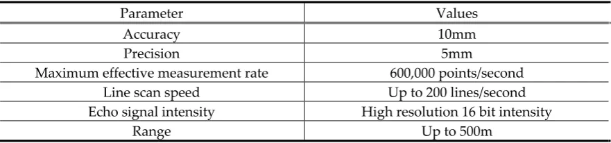
Table 1. Specifications of Trimble MX8 system [28].
Parameter Values
Accuracy 10mm
Precision 5mm
Maximum effective measurement rate 600,000 points/second
Line scan speed Up to 200 lines/second
Echo signal intensity High resolution 16 bit intensity
Range Up to 500m
The length of dataset selected for our study is approximately 1km. There are two pairs of rail tracks and 24 poles at regular intervals. The dataset was divided into 6 sub-regions for the cross-validation purpose, each of which has 4 poles (2 pole-pairs) and its length is approximately 160m. Each sub-region has slightly different configuration of key objects comprising railway electrification systems. In this study, we aim to recognize 10 different classes of railway electrification system objects as shown in Figure 5. The targeted objects play important roles for safely supplying the electricity to the trains. The characteristics of the electrification system objects are represented not only with their geometric saliencies, but also with horizontal and vertical relations among the objects in the railway corridor scene. A brief description of the targeted object classes is given below:
• Electricity feeder (class 1): a set of electric conductors that originate from a primary distribution center and supply power to one or more secondary distribution centers. The electricity feeders are located at the top of railway scene with an elevation of 8 m above the ground (vertical configuration), while they are horizontally placed between rail tracks and poles (horizontal configuration);
• Catenary wire (class 2): a wire to keep the geometry of contact wires within defined limits. The catenary wires are in an elevation of approximately 6.5 m above rails and approximately 1.2 m above contact wire (vertical configuration). In horizontal configuration, the wire is located just above rails;
• Contact wire (class 3): a wire which transfers electrical energy to the train and directly contacts with train. In vertical configuration of railway scene, this wire is in elevation of approximately 5.3m above rails;
• Current return wire (class 4): a wire observed outside rails in horizontal configuration and supported by pole. The current return wires are located between catenary wire and contact wire in vertical configuration;
• Suspension insulator (class 6): a structure connecting between electricity feeder and pole which is observed at the top of railway scene. Note that suspension insulator and a structure attached to pole are defined as class "suspension insulator";
• Movable bracket (class 7): a movable structure attached to pole which supports wires;
• Dropper (class 8): a vertical wire connecting between catenary wire and contact wire;
• Pole (class 9): a pole is located outside of rail tracks and track beds; and
• Ground (class 10): a ground surface placed underneath the overhead wires and rail tracks;
(a) (b)
Figure 5. Electrification system configuration and 10 object classes of Honam high-speed railways illustrated in: (a) a photograph and (b) MLS data.
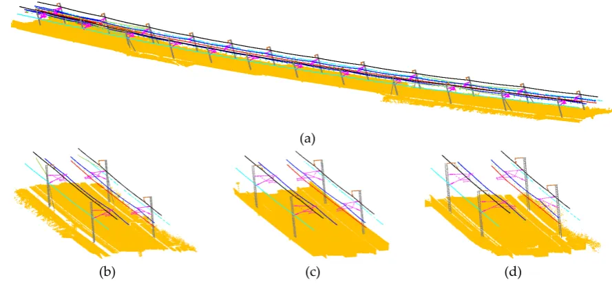
The reference data labeled with 10 object classes was produced by a manual classification method provided by a commercial software, TerraScan. Figure 6 shows the results of the manually labelled reference data. In Figure 6, major overhead wires (i.e., contact and catenary wires) and associate structures (i.e., poles, suspension insulators and brackets) have relatively strong regularities of object layout and appearance. However, some scenes such as sub-region 6 and sub-region 6 in Figure 6 show more complex object configurations where the aforementioned layout regularity is not directly applicable; the sub-regions contains many merging wires and double contact/catenary wires (not single). Also contact wire is often not observed at the one side of railway.
(a)
(e) (f) (g)
Figure 6. Manually classified reference data: (a) entire region, and (b)~(g) six sub-regions (Different colors represent different classes).
4.2 Line extraction results
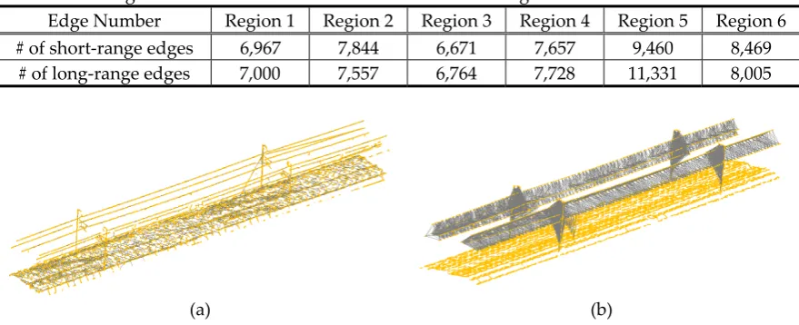
Instead of classifying the entire laser point space, our classification process determines object labels to lines where their member points are classified with the same classes. This line-based classification is suitable for classifying railway corridor scenes, as many key objects (i.e., wires and poles) can be well represented with linear primitives. For converting the laser point clouds (Figure 7(a)) into the line space, we represent the railway corridor scene with voxels with 1 m bin size (Figure 7(b)) and line segments were extracted per voxel using a conventional RANSAC algorithm (Figure 7(c)). Table 2 shows the total number of lines extracted from each sub-region. Note that the RANSAC-based method works iteratively until a termination condition (point residual with respect to corresponding line) is met, which allows extracting multiple line segments with a voxel. Due to the scene complexity, a relatively larger number of lines were extracted in sub-region 5 and sub-region 6.
Table 2. Extracted lines for each sub-region.
Sub-region Region 1 Region 2 Region 3 Region 4 Region 5 Region 6
# of extracted lines 4,327 4,427 3,783 4,091 4,730 4,762
(a) (b) (c)
Figure 7. Example of voxelization and line extraction: (a) input MLS data and rail vectors, (b) voxelization, and(c) extracted lines.
4.3 Classification results
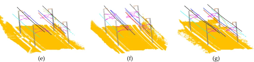
simplify the graph complexity which can significantly accelerate inference speed. Table 3 shows the number of edges generated in each sub-region. Figure 8(a) and 8(b) show the examples of short-range and long-range graphs respectively. In horizontal CRF model, horizontal angle difference, vertical angle difference and difference of horizontal distances between two nodes were used as features while, in the vertical CRF model, height difference between two nodes was used as feature. For the integrated CRF model, multivariate Gaussian parameters in long-range pairwise terms were estimated by maximum likelihood algorithm while the weight parameters for four sub-terms in CRF model were estimated by SGD algorithm as described in Section 3.1. To ensure the stable convergence, the learning rate in SGD starts at 0.0001 and it will halve with the increase of iterations. For the vertical and horizontal long-range pairwise terms, the learning rate is always half of the short-range term because the gradient is steeper for long-range term. Under this setting, we can make sure all weights can converge together.
Table 3. Edge number of different models in different sub-regions.
Edge Number Region 1 Region 2 Region 3 Region 4 Region 5 Region 6
# of short-range edges 6,967 7,844 6,671 7,657 9,460 8,469
# of long-range edges 7,000 7,557 6,764 7,728 11,331 8,005
(a) (b)
Figure 8. Examples of (a) short-range graph and (b) long-range graph.
In this paper, a confusion matrix, also known as an error metric, was used to evaluate the performance of classification methods by comparing our results with reference data. Based on the confusion matrix, precision, recall and F1 score were also calculated for each single class as follows:
=
+ × 100
=
+ × 100
1 = 2 × ×
+
(15)
where TP, FP and FN are true positive, false positive, and false negative, respectively. The precision measures the fraction of the number of true positive prediction of a certain class from the total number of positive class predicted. Recall measures the percentage of the number of true positive prediction of a certain class from the total number of the class in the reference. F1 score is the harmonic mean of precision and recall which reflects the classification quality of a certain class. The classification performance measured by Eq. (5) for three classifiers are presented in Table 4, 5 and 6 respectively. A comparative analysis of three classifiers is summarized in Table 7.
4.3.1 SVM classification results
and recall indicate that electricity feeder, catenary wire, contact wire, current return wire and ground were significantly well classified with over 99% accuracy. However, some misclassification errors mainly occurred over non-major wire objects including suspension insulator, movable bracket, dropper and pole. In particular, relatively low recalls for those classes are observed compared to their corresponding precisions. Many suspension insulators in the reference were classified to poles; movable bracket in the reference was misclassified to various classes such as suspension insulator, dropper, pole and ground in SVM results; many poles in the reference were classified to ground in classified results; some droppers in the reference were classified to movable bracket or pole in classified results (Figure 9).
In this study, line segments were used to extract the features characterizing object saliency. Due the noises involved in MLS data and occlusions, the lines were easily fragmented, which are not sufficient for representing the objects in their full object scale; only local object characteristics can be represented with extracted lines. Thus, similar feature distributions can be found in different objects, which can lead to degraded classification results.
Table 4. Confusion matrix for SVM results: electricity feeder (class 1), catenary wire (class 2), contact wire (class 3), current return wire (class 4), connecting wire (class 5), suspension insulator (class 6), movable bracket (class 7), dropper (class 8), pole (class 9) and ground (class 10).
Classified Recall
(%)
1 2 3 4 5 6 7 8 9 10
Reference
1 1,249 0 0 0 2 0 0 0 0 0 99.84
2 0 1,365 0 0 4 0 2 0 0 0 99.56
3 0 1 687 0 2 0 1 0 0 1 99.28
4 0 0 0 970 0 0 1 0 0 0 99.90
5 0 8 0 0 372 0 12 0 6 6 92.08
6 0 0 0 0 0 73 15 0 16 5 66.97
7 1 1 0 6 7 12 375 12 8 11 86.61
8 0 0 0 0 0 0 4 134 5 1 93.06
9 0 0 0 0 2 6 9 1 678 69 88.63
10 0 0 0 0 0 0 2 0 46 19,932 99.76
Figure 9. Examples of errors caused by SVM: A) suspension insulator in reference was classified to ground, B) movable bracket in reference was classified to ground, C) pole was classified to ground, and D) dropper in
reference was classified to pole.
4.3.2 Classification results for short-range CRF model
The classification results of short-range CRF was summarized in Table 5. Compared to SVM results (Table 7), the major improvements of classification accuracy were attained by the short-range CRF over suspension insulator (+10%), droppers (+2.35%) and movable brackets (+1.07%) in F1 score. Similarly, the short-range CRF improved the classification performance in both precision and recall measures, over suspension insulator and dropper: +10.99% and +3.28% in precision; +9.18% and +1.34% in recall, respectively. While, over movable bracket, +2.07% recall was improved by the short-range CRF, but shows similar performance in precision. These improvements were accomplished by the enforcement of local labeling smoothness implemented using Pott model in the short-range CRF (Section 2.4). In this design scheme, two nodes connected in the short-range graph are likely to have same class. Figure 10 describes the effect of local smoothness. Compare to SVM results (Figure 10 (a)), short-range CRF results present more consistent classification results (Figure 10(b)). For instance, lines belonging to three poles (red circles in Figure 10), which were misclassified with various classes in SVM results, were consistently classified to pole. The results in Table 5 and 7 show that the misclassification errors produced by a local classifier such as SVM can be effectively rectified by only considering the local homogeneous prior as a labeling constraint.
(a) (b)
Figure 10. Effects on short-range CRF: a) SVM results and b) short-range CRF results.
Table 5. Confusion matrix for short-range CRF: electricity feeder (class 1), catenary wire (class 2), contact wire (class 3), current return wire (class 4), connecting wire (class 5), suspension insulator (class 6), movable bracket (class 7), dropper (class 8), pole (class 9) and ground (class 10).
Classified Recall
(%)
1 2 3 4 5 6 7 8 9 10
Reference
1 1,249 0 0 0 2 0 0 0 0 0 99.84
2 0 1,365 0 0 4 0 2 0 0 0 99.56
3 0 0 688 0 2 0 1 0 0 1 99.42
4 0 0 0 970 0 0 1 0 0 0 99.90
5 0 30 0 0 349 0 17 0 4 4 86.39
6 0 0 0 0 0 83 14 0 11 1 76.15
7 0 2 0 6 7 8 384 8 13 5 88.68
8 0 0 0 0 0 0 3 136 5 0 94.44
9 0 0 0 0 2 0 6 0 612 145 80.00
10 0 0 0 0 0 0 3 0 17 19,960 99.90
Precision (%) 100 97.71 100 99.39 95.36 91.21 89.10 94.44 92.45 99.22 98.76
Figure 11. An example of errors produced over connecting wires (green) shown in top view (sky blue: current return wire, black: electricity feeder, blue: catenary wire, red: contact wire, brown: suspension insulator,
magenta: movable bracket, grey: pole).
4.3.3 Classification result for multi-range CRF model
In order to consider layout regularity, the long-range CRF is added to multi-range CRF model. Look-up table and multivariate Gaussian distribution parameters were trained from the training data (Section 3.2.1). In the multi-range CRF model, the weight parameters for different terms in Eq. (3) was
estimated using SGD algorithm (Section 3.1). The weight of unary term (λ) was fixed to 1 and other
three weight values (α,β and γ) were trained using SGD algorithm. The maximum number of
iteration was fixed to 250. Figure 12 shows the transition of weight values according to iterations. The
weight for short-range term α slightly increased and quickly converged to a little higher value than
Figure 12. Weight learning of multi-range CRF model using SGD algorithm.
Once weight parameters were learned, the multi-range CRF was applied. Table 6 describes confusion matrix measuring the classification performance of the multi-range CRF and Table 7 presents its comparative performance analysis to the results of SVM and short-range CRF. As in Table 6, the overall accuracy of the multi-range CRF is 99.44%, which is higher than SVM results (98.91%) and short-range CRF (98.76%). The same conclusion can be read in Table 7, where the multi-range CRF achieved the highest accuracy in F1 score over the most of object classes compared to the other classification results. Moreover, the multi-range CRF shows the least variance in all three performance indices (F1 score, precision and recall) over all ten classes, where the minimum values for these three indices are estimated as 93.43% (connecting wire), 93.14% (pole) and 90.28% (dropper) respectively (Table 7). In F1 score, the most improvements were achieved over following four classes compared to both SVM and short-range CRF: suspension insulator (+23.23%, +13.23%), movable bracket (+6.55, +5.48), dropper (+2.8%, +0.45%) and pole (+6,37%, +9,57%). Those four objects produced major misclassification errors by SVM and short-range CRF.
The most gains achieved by the long-range CRF come from its discriminative ability improved by enforcing spatial layout regularities (horizontal and vertical layout compatibility) among objects. For instance, all movable bracket, which were misclassified to dropper in SVM results, were rectified by the range CRF (Figure 13(a)). It is due to the fact that the horizontal layout term in the long-range CRF utilizes the placement relations of droppers to the rail track and movable bracket in horizontal direction, which shows a strong regular pattern (i.e., dropper is closer to the railway vector than movable bracket in horizontal direction). Also, poles, which were misclassified to ground (c.f., Figure 10) in short-range CRF, were well refined (Figure 13(b)). With similar reason to the dropper case, the misclassification errors over pole class can be rectified by utilizing the horizontal layout compatibility between the rail track and pole (i.e., pole is always observed at the farthest position from the rail track in horizontal direction). In contrast to the horizontal regularity, suspension insulator and movable brackets were significantly improved in both precision and recall by enforcing their vertical regularities in the long-range CRF (Figure 13(c)).
In this experiment, we demonstrate that the multi-range CRF can achieve significant improvement to the classification results obtained by SVM and short-range CRF. However, we found its performance still needs to be further improved, especially over connecting wire and dropper. Both recall and precision for connecting wire were degenerated as shown in Table 6. This degeneracy is caused by a locality of line segment used for characterizing the spatial layouts. If a set of fragmented line segments are extracted from a single connecting line, their distributions in horizontal locations vary, which leads to the ambiguity of encoding the horizontal layout characteristics between connecting lines and other objects. Also, the recall of dropper was lowered. It is due to the fact that contact wire is missing at certain regions so that the relation between dropper and contact wire does not follow the defined vertical regularity. These problems can be potentially resolved by encoding the layout regularities with primitives adaptive to object scales and enlarging training samples.
Classified Recall (%) 1 2 3 4 5 6 7 8 9 10
Reference
1 1,244 0 0 0 7 0 0 0 0 0 99.44
2 0 1,366 0 0 2 0 1 0 2 0 99.64
3 0 2 684 0 3 0 1 0 2 0 98.84
4 0 0 0 970 1 0 0 0 0 0 99.90
5 0 8 14 7 370 0 1 0 4 0 91.58
6 0 0 0 0 0 102 0 0 7 0 93.58
7 0 3 0 11 4 0 411 0 4 0 94.92
8 0 0 0 0 0 0 6 130 8 0 90.28
9 0 0 0 0 1 1 16 0 747 0 97.65
10 0 0 0 0 0 0 2 0 28 19,950 99.85
Precision (%) 100 99.06 97.99 98.18 95.36 99.03 93.84 100 93.14 100 99.44
(a)
(b)
(c)
Figure 13. Visualization of label transitions: (a) dropper in SVM results (left) was classified to movable bracket in integrated CRF model (right); (b) ground in short-range CRF (left) was classified to pole in integrated CRF model (right); (c) suspension insulators were well rectified in integrated CRF model (right).
effect on improving classification results of SVM classifier, particularly rectifying elements which have strong spatial regularity.
Figure 14. Label transition from SVM to integrated CRF: EF (Electricity Feeder), CAW (Catenary Wire), COW (Contact Wire), CNW (Current Return Wire), SI (Suspension Insulator), MB (Movable Bracket), Dro (Dropper),
Pol (Pole) and Gro (Ground).
The performances including precision, recall, and F1-score of three different classifiers were compared in Table 7. Classification results for four types of transmission lines, which are relatively well classified in SVM and short-range CRF, remain at the similar level of accuracy in the proposed multi-range CRF. However, suspension insulator, movable bracket, pole and ground were significantly improved. This result indicates that our proposed multi-range CRF can well improve SVM results, particularly for minor railway elements less occurred in railway scene.
Table 7. The comparison of three different classifiers
Class
SVM Short-range CRF Multi-range CRF
Recall (%)
Precision (%)
F1 score (%)
Recall (%)
Precision (%)
F1 score (%)
Recall (%)
Precision (%)
F1 score (%)
Electricity feeder 99.84 99.92 99.88 99.84 100 99.92 99.44 100 99.72
Catenary wire 99.56 99.27 99.41 99.56 97.71 98.63 99.64 99.06 99.35
Contact wire 99.28 100 99.63 99.42 100 99.71 98.84 97.99 98.42
Current return wire 99.90 99.38 99.64 99.90 99.39 99.64 99.90 98.18 99.03
Connecting wire 92.08 95.63 93.82 86.39 95.36 90.65 91.58 95.36 93.43
Suspension insulator 66.97 80.22 73.00 76.15 91.21 83.00 93.58 99.03 96.23
Movable Bracket 86.61 89.07 87.82 88.68 89.10 88.89 94.92 93.84 94.37
Dropper 93.06 91.16 92.09 94.44 94.44 94.44 90.28 100 94.89
Pole 88.63 89.33 88.97 80.00 92.45 85.77 97.65 93.14 95.34
Ground 99.76 99.54 99.64 99.90 99.22 99.56 99.85 100 99.92
Average 92.57 94.35 93.39 92.43 95.89 94.02 96.57 97.66 97.07
5. Discussion
In this paper, we proposed a new multi-range CRF model to classify railway scene which can consider vertical and horizontal object relations in railway scene as well as local smoothness. The experimental results over 6 datasets showed that better classification accuracy was achieved compared to SVM results. More specifically, experimental results are summarized as follows:
• Short-range CRF plays an important role in improving misclassified lines produced by SVM,
which was achieved by enforcing local smoothness;
• Horizontal long-range CRF shows its performance in correcting railway elements which have
and short-range CRF, were well classified because the element has distinct spatial relations compared to other elements in horizontal layout compatibility;
• Vertical long-range CRF play a major role in refining railway elements such as suspension
insulator, movable bracket, and ground whose vertical regularity is obvious;
• The experimental results showed that the proposed multi-range CRF model can well refine
misclassified errors in local classifier if there are strong regularity among railway elements. Compared to SVM results, both precision and recall of suspension insulator, movable bracket, pole and ground were improved. Also, the accuracies for electronic feeder, catenary wire, contact wire and current return wires, which were well classified in SVM, still remain a similar level of accuracy. However, the classification performance of dropper and connecting wire decrease was degenerated due to the layout ambiguity;
• The line-based graph model shows its effectiveness for representing railway electrification
system objects and provides computation efficiency. However, locally extracted line segments show their limitations in representing objects with their full scales, which causes problems in characterizing the short-range and long-range regularities and thus lead to misclassification errors.
As future work, we will explore the potential of multi-scale line segments holistically representing object characteristics and construct graphical models. Also, we will evaluate the proposed multi-range CRF over a range of railway scenes which have different configurations. In addition, the proposed CRF model will be extended by applying new regularities which are observed in railway scene or by considering a hierarchical CRF model. For instance, poles are located at regular interval and the relation can be represented by very long-range graph or at a different scale.
Acknowledgments: This research was supported by a grant (15RTRP-B067297-03) from Railroad Technology Research Program (Technology development on the positioning detection of railroad with high precision) funded by Ministry of Land, Infrastructure and Transport of Korea government.
Author Contributions: G.S initiated current research project as a principal investigator and have supervised the research works conducted by J.J. and L.C. J.J. L.C. and G.S. conceived and designed the experiments; J.J and L.C. contributed with the experimental work and data analysis; C.L. dedicated his valuable suggestions on model design; J.W dedicated comments on railway infrastructure; J.J, L.C and G.S wrote the paper.
References
1. U.S. Department of Transportation. https://www.transportation.gov/ (accessed on 18 September, 2016). 2. Arastounia, M. Automated recognition of railroad infrastructure in rural areas from lidar data. Remote
Sensing2015, 7, 14916-14938.
3. Oura, Y.; Mochinaga, Y; Nagasawa, H. 1998. Railway electric power feeding systems. Japan Railway & Transport Review1998, 16, pp. 48-58.
4. Zhang, S.; Wang, C.; Yang, Z.; Chen, Y.; Li, J. Automatic railway power line extraction using mobile laser scanning data, In Proceedings of the International Archives of the Photogrammetry, Remote Sensing and Spatial Information Sciences, Prague, Czech Republic, 12-19 July 2016; Volume XLI-B5, pp. 615-619. 5. Jwa, Y.; Sohn, G. Kalman filter based railway tracking fr*785220om mobile lidar data. In Proceedings of the
ISPRS Annals of the Photogrammetry, Remote Sensing and Spatial Information Sciences, La Grande Motte, France, 28 September – 3 October 2015; Vol II-3/W5, pp. 159-164.
6. Niemeyer, J.; Rottensteiner, F.; Soergel, U. Contextual classification of lidar data and building object detection in urban areas. ISPRS Journal of Photogrammetry and Remote Sensing2014, 87, pp. 152-165.
7. Luo, C.; Sohn, G. Scene-layout compatible conditional random field for classifying terrestrial laser point clouds. The ISPRS Annals of the Photogrammetry, Remote Sensing and Spatial Information Sciences, Zurich, Switzerland, 5-7 September 2014; Volume II-3, pp. 80-86.
8. Muhamad, M.; Kusevic, K.; Mrstik, P.; Greenspan, M. 2013. Automatic rail extraction in terrestrial and airborne LiDAR data, Proceedings of the 2013 International Conference 3D Vision, Seattle, USA, 29-30 June 2013; pp. 303-309.
10. Guo, B.; Li, Q.; Huang, X.; Wang, C. An improved method for power-line reconstruction from point cloud data, Remote Sens.2016, 8, 36.
11. Chehata, N.; Guo, L.; Mallet, C., 2009 Airborne lidar feature selection for urban classification using random forests, In Proceedings of the International Archives of the Photogrammetry, Remote Sensing and Spatial Information Sciences, Paris France, 1-2 September 2009; Volume XXXVIII (Part 3/W8), pp. 207-212. 12. Zhang, J.; Lin, X.; Ning, X. Svm-based classification of segmented airborne lidar point clouds in urban areas.
Remote Sensing 2013, 5, 3749-3775.
13. Lafarge, F.; Mallet, C. Creating large-scale city models from 3d-point clouds: a robust approach with hybrid representation. International Journal of Computer Vision2012, 99, pp. 69-85.
14. Kohli, P.; Torr, P.H. Robust higher order potentials for enforcing label consistency. International Journal of Computer Vision 2009, 82, 302-324.
15. Nowozin, S.; Rother, C.; Bagon, S.; Sharp, T.; Yao, B.; Kohli, P. Decision tree fields. 13th International Conference on Computer Vision, Barcelona, Spain, 6-13 November 2011; pp. 1668-1675.
16. Lim, E. H.; Suter, D. 3d terrestrial lidar classifications with super-voxels and multi-scale conditional random fields. Computer-Aided Design 2009, 41, 701-710.
17. Winn, J.; Shotton, J. The layout consistent random field for recognizing and segmenting partially occluded objects, 2006 IEEE Computer Society Conference on Computer Vision and Pattern Recognition, New York, USA, 17-22 June 2006; pp 37-44.
18. Gould, S.; Rodgers, J.; Cohen, D.; Elidan, G.; Koller, D. Multi-class segmentation with relative location prior.
International Journal of Computer Vision 2008, 80, 300-316.
19. Kumar, S.; Hebert, M. Discriminative random fields. International Journal of Computer Vision2006, 68(2), pp. 179-201.
20. Shotton, J.; Winn, J.; Rother, C.; Criminisi, A. Textonboost for image understanding: Multi-class object recognition and segmentation by jointly modeling texture, layout, and context. International Journal of Computer Vision 2009, 81, 2-23.
21. He, X.; Zemel, R. S.; Carreira-Perpiñán, M. A. Multiscale conditional random fields for image labeling, Proceedings of the 2004 IEEE Computer Society Conference on Computer Vision and Pattern Recognition (CVPR’04), Washington, DC, USA, 27 June – 2 July 2004; pp. 695-702.
22. Douillard, B.; Fox, D.; Ramos, F. Laser and vision based outdoor object mapping. Robotics: Science and Systems IV, Zurich, Switzerland, 25-28 June, 2008.
23. Lodha, S. K.; Kreps, E. J.; Helmbold, D. P.; Fitzpatrick, D.N. Aerial lidar data classification using support vector machines (svm), 3DPVT 2006, Chapel Hill, USA, 14-16 June 2006; pp 567-574.
24. Schindler, K. An overview and comparison of smooth labeling methods for land-cover classification. IEEE Transactions on Geoscience and Remote Sensing 2012, 50, 4534-4545.
25. Gauvain, J. L.; Lee, C. H. Maximum a posteriori estimation for multivariate gaussian mixture observations of markov chains. IEEE transactions on speech and audio processing 1994, 2, 291-298.
26. Gardner, W.A. Learning characteristics of stochastic-gradient-descent algorithms: A general study, analysis, and critique. Signal Processing 1984, 6, 113-133.
27. Bowling, M.; Veloso, M. Multiagent learning using a variable learning rate. Artificial Intelligence 2002, 136, 215-250.
28. Trimble MX8 Datasheet. https://www.trimble.com/imaging/pdf/Trimble_MX8_Datasheet.pdf (accessed on 18 Sep 2016).