Article
River Water Quality: Who Cares, How Much and
Why?
Danyel Hampson 1, Silvia Ferrini 2, Dan Rigby 3 and Ian J. Bateman 4,*
1 Land, Environment, Economics and Policy Institute (LEEP), University of Exeter, Exeter, EX4 4PJ, UK; [email protected]
2 Centre for Social and Economic Research on the Global Environment, School of Environmental Sciences, University of East Anglia, Norwich Research Park, Norwich, Norfolk, NR4 7TJ, UK and Department of Political Science and International, University of Siena 1240, 10. Mattioli, 53100 Siena, Italy; [email protected]
3 Department of Economics, University of Manchester, Manchester, M13 9PL, UK; [email protected]
4 Director, Land, Environment, Economics and Policy Institute (LEEP), University of Exeter, Exeter, EX4 4PJ, UK; [email protected]
* Correspondence: [email protected]; Tel.: +44-01392-724503 ext. 4503
Abstract: One important motivation for the implementation of the Water Framework Directive is the creation of non-market environmental benefits such as improved ecological quality, or greater opportunities for open-access river recreation via microbial pollution remediation. Pollution sources impacting on ecological or recreational water quality can be uncorrelated but non-market benefits arising from riverine improvements are typically conflated within benefit valuation studies. Using stated preference choice experiments, we seek to disaggregate these sources of value for different river users, thereby allowing decision makers to understand the consequences of adopting alternative investment strategies. Our results suggest anglers derive greater value from improvements to the ecological quality of river water, in contrast to swimmers and rowers for whom greater value is gained from improvements to recreational quality. We also find three distinct groups of respondents: a majority preferring ecological over recreational improvements, a substantial minority holding opposing preference orderings and a small proportion expressing relatively low values for either form of river quality enhancement. As such, this research demonstrates that the non-market benefits which may accrue from different types of water quality improvements are nuanced in terms of their potential beneficiaries and, by inference, their overall value and policy implications.
Keywords: Water Framework Directive; ecological and microbiological water quality; choice experiment; willingness to pay for river water quality; conditional logit; latent class analysis; non-market benefits
1. Introduction
The Water Framework Directive (WFD) requires substantial improvements to the quality of Europe’s waters so that the ‘good ecological status’ of surface waters is achieved [1]. One important motivation for the implementation of the WFD appears to be the creation of non-market social benefits such as improved provision of, and opportunities for, open-access recreation (Articles 4, 9 and 11 of the WFD).
Previous research has shown that it is technically infeasible and prohibitively expensive for all UK rivers to be brought to ‘good ecological status’ within the near future [2]. The WFD allows derogations from ‘good ecological status’ where remediation projects may be technically infeasible or remediation costs may be disproportionate to the benefits created (article 4, par. 4, 5, 7). The financial costs of pollution remediation must be offset against the benefits of that remediation. Some benefits may be measured on the market and are commonly accounted for in water management
plans [3]. Official UK guidelines state that non-market costs and benefits must not be ignored but must be ‘quantified where possible and meaningful’ [4]. Therefore the role of economics is crucial in assessing the non-benefits of measures which could be implemented to achieve WFD targets, as these benefit values may represent significant components of water quality improvements [5].
Among economic valuation techniques, stated preference methods have been extensively used for valuing the non-market benefits arising from environmental improvements, with choice experiments (CE) used since the late 1990s for water quality studies. This trend has continued over the last ten years, with the method used to assess a diverse range of water quality issues including assessments of wetland conservation projects [6], multi-country assessments of benefit transfer in water conservation projects [7] and adaptations to river use [8].
Valuation studies typically assess WFD benefits in ways which conflate the value of ecological improvements with the value of microbial pollution reduction, therefore assessing water quality as a single attribute of preference [9,10]. However, the ecological and microbial attributes of water are not identical. They are affected differently by different pollutants and different benefits accrue from remediation measures designed to reduce either type of pollution. Ecological quality is relevant for conservation/biodiversity and is principally determined by diffuse nutrient pollution (e.g. nitrates and phosphates) from agriculture, while microbiological quality is relevant for recreation1 and is
largely determined by faecal pollution, typically from livestock and/or wastewater treatment works [12]. Doherty et al. [13] observe that ‘a consequence of focusing on just the ecological status of the water bodies being analysed is that the marginal value of a specific characteristic of a waterbody (e.g. the marginal value of a change in the recreational or aesthetic attribute) cannot be estimated’.
In the UK, the most recent CE water quality studies include Hanley et al. [14], Glenk et al. [10], Metcalfe et al. [15] and Doherty et al. [13]. Hanley et al. provide willingness to pay (WTP) measures for improvements from fair to good for ecological quality, aesthetic and bankside condition attributes of the rivers Wear (Durham) and Clyde (Central Scotland). Glenk et al. and Metcalfe et al. describe the state of water bodies (rivers and lochs in the former and all water bodies in the latter) and assess respondents’ preferences for the potential future status of those water bodies. Doherty et al. disentangle water quality characteristics into aquatic ecosystem health, water clarity and odour attributes. None of these studies sought to separate the microbiological/recreational component of water quality from the ecological attribute.
This research furthers the knowledge on non-market valuation of river water by disaggregating the values which people derive from ecological and microbial aspects of river water quality. Given the link between microbial quality and recreational river use we investigate how the values for these distinct attributes of river water quality differ over people who (i) engage with the river in different ways (rowers, swimmers, anglers) and (ii) who live at different distances from the river. This investigation is undertaken using a stated preference, Discrete Choice Experiment (DCE), with discrete attributes for ecological and recreational water characteristics.
Our results indicate significant heterogeneity in water quality preferences: a majority of respondents prefer ecological improvements, a substantial minority prefer recreational improvements, and a small proportion hold relatively low values for either form of river quality enhancement. Anglers prioritise ecological quality, swimmers and rowers favour improved recreational opportunities. A clear distance decay in respondents’ WTP values away from the site of proposed investment was revealed. As such this research demonstrates that the non-market benefits which may accrue from different types of water quality improvements are nuanced in terms of their environmental impacts, their potential beneficiaries and, by inference, their overall value and policy implications. This information allows decision makers to better understand the consequences of
1
Microbiologically polluted water has been shown to have a dose-response relationship with the
risk of ill-health. Reducing the risk of ill-health via microbial pollution reduction leads to improved
adopting alternative investment strategies which favour either ecological or recreational improvements, or a mix of benefits, as these trade-offs were previously poorly understood [16].
2. Materials and Methods
2.1. Case study area and catchment
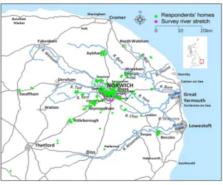
The survey was conducted in Norfolk, UK. The River Yare was selected as a case study area to study ecological and recreational values as the Yare catchment is prone to diffuse agricultural nutrient pollution, having been designated as a Catchment Sensitive Farming priority [17], and has difficulties meeting WFD targets due to pollution from the water industry [18]. Figure 1 shows the survey area, the locations of respondents’ homes and the 20km survey stretch of the River Yare.
Figure 1. The survey area, survey river stretch and spatial distribution of respondents.
2.2. Survey instruments and choice experiment design
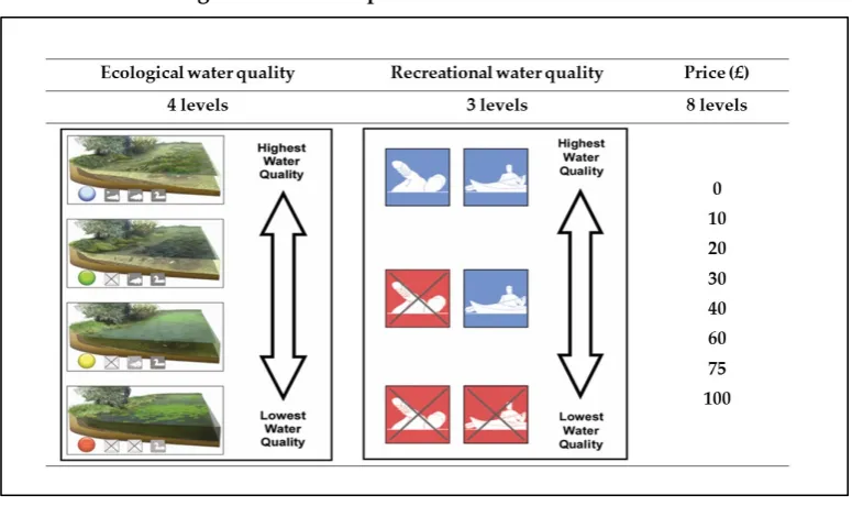
Water quality ladders (graphical indices of scientifically quantified parameters) are extensively used to convey information to respondents. Unfortunately, a common characteristic of these ladders is that they conflate ecological and microbiological quality attributes [19]. We disaggregate the water quality ladder developed by Hime et al. [20] into ecological and recreational components. To sufficiently address our research question, yet minimise the cognitive load on respondents, we use three simple attributes to describe water quality across a range of future water quality scenarios at the survey river stretch (Figure 2). Ecological quality has four levels ranging from ‘blue’ (the highest) to ‘red’ (the lowest). These levels are based on UKTAG guidance [21]. Recreational quality has three levels; ‘high’, ‘medium’ and ‘low’. Price has eight levels ranging from £0 to £100. The payment vehicle was presented as a hypothetical increase to respondents’ annual domestic water bill.
little or no resemblance to reality [22,23]. This divergence can reduce the accuracy of welfare estimates: Poor et al. [24] demonstrate the impact of objective vs. perceived measures in valuing the water clarity of lakes in Maine. This study circumvents these issues in two ways. We collect the perceptions of water quality directly from respondents and incorporate those perceptions into welfare benefit valuations. We also use a forced choice design in which there is no “status quo” opt out option included in each set. The absence of a “current” option reflects the reality of water management in the context of the study: the status quo is not an option due to the implementation of WFD induced water quality improvement programmes. Forced choice designs have been used in other water DCE studies where the status quo is no longer an option [25,26]. Welfare analysis is still possible as long as the current levels of the attributes are included in the experimental design. Questions to capture other variation in WTP (e.g. distance, respondents’ socio-economic characteristics and use patterns) were included elsewhere within the survey.
Figure 2. Choice experiment attributes and levels.
A balanced orthogonal experimental design was developed2, conforming to a D-efficient
design3, within a conditional logit (CL) framework with fixed efficiency measures to maximize the
parameter precision. Combining the attributes and levels shown in Figure 2, 48 combinations were produced which were arranged into four blocks of twelve choices, with each block presented to 50 respondents, for a total of 200 respondents.
A recruitment strategy was devised which differentiated between river visitors (who deliberately visited rivers within the previous year) and non-visitors and, of those respondents who identified as visitors, captured different recreation types.
2.3. Modelling strategies
2.3.1. Conditional logit modelling
The CL model is frequently used in choice modelling studies to estimate the impact of choice attributes and respondents’ socio-economic characteristics on the utility derived by alternatives [28]. We assume that the respondent compares attributes and attribute levels and chooses the option
2 Experimental design devised using NGene v.1.1 [27].
3
which maximizes utility. Following Random Utility Maximization theory [29], the utility can be formalized as
Uijt =Vijt+ eijt =
β
i xijt +ε
ijt i=1,….,N; j=1,…,J; t=1,…,T (1)where xijt is a K-vector of observed attributes of alternative j facing person i on occasion t, while
β
i isa vector of person i specific utility weights on these attributes and
ε
ijt is the error term.Different assumptions on the error term
ε
ijt lead to alternative modeling strategies. The CL modelassumes Extreme Value Type I error terms [29], and is formalized as
( it= | = ) = ( )
∑ ( ) (2)
In this specification preference heterogeneity can be incorporated in the model by interacting socio-economic variables with choice attributes. CL estimation is carried out with standard maximum likelihood techniques.
Unfortunately, the CL model has several drawbacks [30]. Repeated observations by the same respondents cannot be accommodated by the model and heterogeneity in preference cannot be properly addressed. McFadden and Train [31] provide the LM test, which uses artificial variables to verify heterogeneity in preferences. Dropping the t-index for simplicity, the artificial variables can be obtained as
= ( − ) , with = ∑ (3)
where Pij is the CL choice probability. The CL model in Equation 2 is re-estimated including the
artificial variables and the null hypothesis of no random coefficients on attributes x is rejected if the coefficients for the artificial variables, tested using a Wald or Likelihood Ratio test, is significantly different from zero. An alternative model specification is latent class (LC) which overcomes CL limitations in addressing preference heterogeneity [32] and repeated choices [33].
2.3.2. Latent class analysis
The LC model posits that preferences can be explained by observable and latent factors [34]. The model structure is extended to accommodate unobservable heterogeneity explained by socio-economic characteristics or attitudinal/psychological information [35]. From a policy perspective, Latent class (LC) analysis enables environmental managers to respond more appropriately to the preferences of those subgroups [36]. There has been a growing use of LC to assess environmental preferences, e.g., in recreational angling [37], wilderness recreation [38] and reservoir recreation [39]. Although intra-class respondents may display relatively homogeneous preferences, the functional form of LC places no restrictions on class membership probabilities, allowing for a wider range of preference heterogeneity within a class, thus solving the limitations of IIA on the distribution of the preference parameters. LC also retains the data’s intra-respondent panel structure.
Formally a LC model uses a probabilistic class allocation model and a CL model for the alternative choices. Each respondent i belongs to class s (of S classes) with probability πis, with ∈
(0,1) and ∑ . The probability that respondent i belongs to class s is
=∑ ( ( ) ) (4)
where δs is a class specific constant, zi is a vector of individual socio-economic characteristics and γs
Conditional on the probability of being in class s the probability of choosing option j among the
J alternatives is equivalent to Equation 2. The unconditional probability of choosing option j for respondent i for choice situation t=1 is the product of Equations 4 and 2:
( | ,… , ) = ∑ ( i= | = ) (5)
In common with the CL specification, maximum likelihood procedures can be used to estimate the LC model. Respondents’ individual class membership probabilities were calculated using the method described in Morey and Thacher [40], which enables each respondent to be allocated to their most likely class using that individual’s conditional class-membership probabilities. Post-estimation results were then defined using class members’ socio-economic characteristics.
Following welfare theory [41], both models can provide marginal welfare values by the ratio of marginal utility of each attribute (k) and price (p)
= − |
| (6)
The WTP ratio can be derived when we can observe a marginal change from the initial state of water and a future change. The choice setting deliberately avoided defining the current water quality level (status quo) and the survey collected information on perceived water quality. We estimate WTP in two ways: we use ‘low’ ecological or recreational quality as objective initial water quality states, or, as in Hynes et al. [42], we use perception of water quality. We consider, at the individual level, the perceived water quality and where that respondent’s perception is lower than the improvement, WTP is set to zero (e.g. should we want to improve the river from low to medium water quality, if the respondent’s perception is already medium (or high) the improvement does not produce any benefit.). The marginal WTP is registered for the other cases4. The Krinsky and Robb method [43] of
calculating the confidence interval of WTP estimates was used.
3. Results
3.1. Summary statistics
Table 1. Descriptive statistics.
Whole sample (88 male, 112 female) 200
Rowers and swimmers in sample 15
Anglers in sample 16
Mean number of environmental memberships per respondent 0.5
Mean distance respondents live from the survey river 8km
Mean income £28,600
To examine distance decay effects, respondents were interviewed at a range of distances (0.1-79.4km), from the survey river stretch. To explore preference heterogeneity, a range of respondents were interviewed. 185 respondents from the general public were interviewed either door to door or at the survey river. Swimmers and rowers account for less than 1% of the population but were deliberately oversampled (from local recreation clubs) to generate data for analysis. There were 16 anglers within the sample.
3.2. Conditional logit results
4
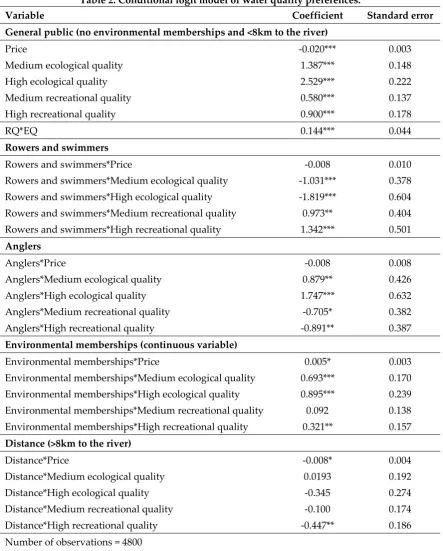
Table 2. Conditional logit model of water quality preferences.
Variable Coefficient Standard error
General public (no environmental memberships and <8km to the river)
Price -0.020*** 0.003
Medium ecological quality 1.387*** 0.148
High ecological quality 2.529*** 0.222
Medium recreational quality 0.580*** 0.137
High recreational quality 0.900*** 0.178
RQ*EQ 0.144*** 0.044
Rowers and swimmers
Rowers and swimmers*Price -0.008 0.010
Rowers and swimmers*Medium ecological quality -1.031*** 0.378
Rowers and swimmers*High ecological quality -1.819*** 0.604
Rowers and swimmers*Medium recreational quality 0.973** 0.404
Rowers and swimmers*High recreational quality 1.342*** 0.501
Anglers
Anglers*Price -0.008 0.008
Anglers*Medium ecological quality 0.879** 0.426
Anglers*High ecological quality 1.747*** 0.632
Anglers*Medium recreational quality -0.705* 0.382
Anglers*High recreational quality -0.891** 0.387
Environmental memberships (continuous variable)
Environmental memberships*Price 0.005* 0.003
Environmental memberships*Medium ecological quality 0.693*** 0.170
Environmental memberships*High ecological quality 0.895*** 0.239
Environmental memberships*Medium recreational quality 0.092 0.138
Environmental memberships*High recreational quality 0.321** 0.157
Distance (>8km to the river)
Distance*Price -0.008* 0.004
Distance*Medium ecological quality 0.0193 0.192
Distance*High ecological quality -0.345 0.274
Distance*Medium recreational quality -0.100 0.174
Distance*High recreational quality -0.447** 0.186
Number of observations = 4800 Log likelihood = -1009.737
*, ** and *** = significance at 10%, 5% and 1% levels.
The CL model5, shown on Table 2, presents preference heterogeneity in the naïve way
(interaction of attributes and socio economic variables) but provides preliminary insights into preference heterogeneity. Respondents’ preferences for Yellow and Green ecological quality levels were insignificantly different from one another so those levels were collapsed into one intermediate
5
variable called Medium ecological quality. For clarity Blue ecological quality is renamed High ecological quality.
The first section of Table 2 displays estimated marginal utilities of the general public (i.e. are not rowers, swimmers or anglers) who are not members of environmental groups and live within 8km of the river. Coefficients for Medium and High ecological, and Medium and High recreational water quality levels are complete and transitive. The strength of the coefficients relative to one another suggests that such respondents, on average, value improvements in ecological quality more than they do improvements in recreational/microbial water quality. Respondents dislike options containing higher prices, ceteris paribus.
An interaction term, RQ*EQ, describes a highly significant positive interaction for all respondents: improvements in one dimension of water quality (whether it be ecological quality or recreational quality) are valued more highly the higher the quality level of the other dimension of water quality.
Membership of environmental organisations is typically used as a surrogate variable to positively identify respondents who would be expected to care more highly about the environment. Within this sample members of environmental organisations have highly significant preferences for higher levels of ecological water quality and hold higher values for High recreational water quality. They are also slightly more likely to choose choice options containing higher prices.
Anglers are significantly more likely to value improved ecological water quality and their preference for High ecological quality is significantly higher than their preference for Medium ecological quality. Anglers had lower preferences (relative to the other respondents) for both levels of recreational water quality but this is reasonable if lower recreational quality reduces the number of people using the river and disturbing the angler and the fish. Conversely, swimmers and rowers are significantly more likely to value improved recreational water quality and significantly less likely to choose options containing higher ecological quality. This is reasonable given that recreational quality is important in order for them to enjoy their activities safely.
The model provides evidence of a step-function distance decay on Price, as respondents who live further than 8km from the river are less willing to choose choice options containing higher prices. With a p-value of 0.054, this coefficient is very close to the 5% significance level. Respondents also hold significantly lower preferences for High recreational quality, if they live farther from the river. This fits the concept that non-use value is less responsive to distance than use value [45].
It may not be the case that the preferences of the different respondents are as one dimensional as the CL model suggests but this has occurred, in part, due to parameterising the model in the most efficient way to best represent the preferences of the different user groups. LM testing verified unexplained heterogeneity within several of the model’s coefficients6 and as CL fails to control for
intra-respondent variation, we conclude that CL is not the optimal specification of the choice data. As the aim of our research is to reveal as much preference heterogeneity as possible, we now turn to the LC analysis.
3.3. Latent class results
Within LC analysis the assumption is that respondents’ behaviour within a choice experiment is a manifestation of their underlying latent preferences. The optimum number of latent classes was tested using the information criteria measures suggested by Hynes et al [42]. The Baysian Information Criteria and the Consistent Akaike Information Criteria indicated that a model containing three classes of respondents was the optimal solution. Respondents are allocated to the three classes reported in Table 3. The LC model7 is composed of two groups of variables. The utility functions
describe the estimated marginal utilities for the choice attributes held by each class. The class
6
Price, High Recreational Quality and RQ*EQ variables have heterogeneous variance within the CL
model.
7
membership covariates capture the impact of observables on class membership probabilities. We discuss each in turn.
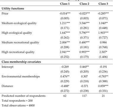
Table 3. Latent class model of water quality preferences.
Class 1 Class 2 Class 3
Utility functions
Price -0.014*** -0.023*** -0.285***
(0.005) (0.003) (0.071)
Medium ecological quality 1.211*** 3.546*** 1.040**
(0.171) (0.281) (0.448)
High ecological quality 1.647*** 5.790*** 1.903***
(0.262) (0.371) (0.727)
Medium recreational quality 2.006*** 0.480*** 0.984
(0.208) (0.181) (0.768)
High recreational quality 2.941*** 0.993*** 2.507*
(0.252) (0.175) (1.406)
Class membership covariates
Intercept -0.269 0.460** -0.191
(0.245) (0.205) (0.236)
Environmental memberships 0.476** 0.307 -0.783**
(0.229) (0.218) (0.388)
Distance -0.488* -0.371 0.859***
(0.272) (0.238) (0.331)
Predicted number of respondents 62 117 21
Total respondents = 200 Total observations = 4800
*, ** and *** = significance at 10%, 5% and 1% levels. Standard errors in parenthesis.
The utility functions reveal significant preference heterogeneity between the 3 classes. Class 1 is estimated to contain 62 respondents. These respondents have the highest utility from improved recreational water quality. Class 2 contains the majority of the respondents (117) and they are most likely to value improved ecological water quality. Class 3 is the smallest class, containing 21 respondents. Although Class 3 respondents hold positive preferences for improved levels of ecological and recreational water quality, they avoid choice options containing increased Price: we see a highly significant (relatively steep) negative slope on the Price coefficient for Class 3.
Variables for the number of Environmental Memberships held by respondents and their Distance from the proposed improvement help define which class respondents were assigned to. As the number of Environmental Memberships increases, respondents are significantly less likely to be assigned to Class 3, and it is highly significantly more likely that respondents will be assigned to Class 3 if they live farther from the river. Post-estimation results (Table 4) show that Class 3 respondents tend to live furthest from the river and hold the lowest number of Environmental Memberships.
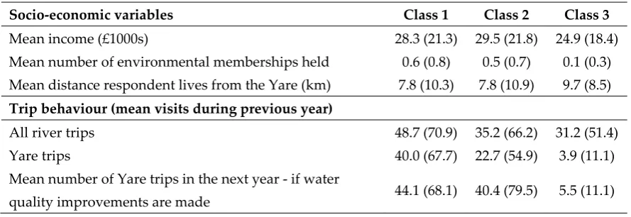
Table 4. Post-estimation results for the latent class model.
Socio-economic variables Class 1 Class 2 Class 3
Mean income (£1000s) 28.3 (21.3) 29.5 (21.8) 24.9 (18.4)
Mean number of environmental memberships held 0.6 (0.8) 0.5 (0.7) 0.1 (0.3)
Mean distance respondent lives from the Yare (km) 7.8 (10.3) 7.8 (10.9) 9.7 (8.5)
Trip behaviour (mean visits during previous year)
All river trips 48.7 (70.9) 35.2 (66.2) 31.2 (51.4)
Yare trips 40.0 (67.7) 22.7 (54.9) 3.9 (11.1)
Mean number of Yare trips in the next year - if water
quality improvements are made 44.1 (68.1) 40.4 (79.5) 5.5 (11.1)
Standard errors in parenthesis.
On average, Class 3 respondents take relatively few trips to the Yare. Respondents were asked about their future trip behaviour and, even if water quality was guaranteed to be high at the Yare, Class 3 respondents’ future trip frequency may barely change. It is likely that Class 3 respondents are unwilling to pay for water quality improvements at the Yare due to a variety of factors, including a preference to visit substitute river locations.
Class 1 respondents’ future trip frequency at the Yare is also relatively inelastic. It seems that although they are willing to pay for improved recreational water quality for others to enjoy at the Yare, they are not keen to make increased use of that resource. This altruistic choice behaviour has been observed in previous research [47]. In contrast, Class 2 respondents are not only willing to pay for ecological water quality improvements, but may also visit far more frequently to enjoy those improvements.
3.4. Willingness to pay for water quality improvements
We now consider the monetary values for WTP, which are derived by assessing changes in utility from V0, the initial water quality state, and V1, the alternative state. Using the correct value for
V0 is crucial, as, if incorrect, the resulting WTP estimates will also be incorrect. For example; if
ecological quality is consistently low it would be correct to set V0 for ecological quality to low.
However, water quality on the Yare isn’t always low, but variable throughout the year, which complicates our attempts to accurately define V0.
Figure 3. WTP derived from the LC model for each water quality type, per km8 of improvement, per household, per year.
There are distinct difference in WTP between the different classes. Class 1 respondents hold the highest values for recreational improvements, Class 2 respondents value ecological water quality enhancements more highly and Class 3 respondents have very low values for either water quality attribute.
We believe that the most important factor influencing the correct level of V0 in situations where
V0 is variable, or where there is no correct level of V0, is the respondent’s own perception of existing
water quality. For this reason, we recalculate WTP estimates for each individual, with V0 set to the
level of water quality perceived by that individual.
Within the survey the current state of the water quality was not fixed and was intentionally overlooked in the CE setting. Instead, Yare visitors were asked what quality they thought each attribute was at the Yare and their perceptions are shown in Figure 4. We see a small minority who believe that the existing water quality is Low, while the remainder think that water quality is Medium or High. Non-visitors, unable to provide perceptions data, are excluded from the following analysis.
Figure 4. Visitors perceptions of current water quality at the Yare.
Within Table 5 we see that where V0 is set to the lowest water quality level, WTP estimates are
much higher than if we use respondents’ perceptions of water quality as the baseline upon which to calculate welfare estimates. It is important that we use the correct level for V0 to produce meaningful
8
valuations: if V0 is systematically set to the lowest water quality level WTP estimates are potentially
overestimated.
Table 5. WTP of Yare visitors (excluding rowers and swimmers) per km of improvement, per household, per year, accounting for perceived water quality.
Improvement type If V0 = low water quality if V0 = respondent’s perception
Medium ecological quality £5.27 £0.37
High ecological quality £8.36 £1.15
Medium recreational quality £2.15 £0.10
High recreational quality £3.51 £0.40
4. Discussion
This research disentangles and examines the relationships between ecological and recreational sources of value, thereby allowing decision makers to better understand the consequences of adopting alternative investment strategies which favour either ecological, recreational or a mix of benefits. To do this, this research has used attribute based valuation methods and a broad survey design to analyze the way in which individuals regard the recreational and environmental functions of rivers. We present two complementary models which examine different aspects of the same data. With regard to the question of who cares about river water quality, our results are stable over the alternative choice models specifications, confirming significant heterogeneity in water quality preferences across the sample of respondents. Clearly the answer to ‘Who cares?’ depends on who is being asked, and asked for what reason. Previous research led us to expect that recreational water users would have higher expectations from water quality in order to fully enjoy their activities and would place greater value on higher recreational water quality. This expectation is confirmed within our CL results, which provide an overview of the water quality preferences of different recreational users and infrequent visitors/non-users within the general public. The public held higher values for improved ecological quality, rather than recreational enhancements. Similar preference orderings, but at higher levels of willingness to pay, were revealed by anglers. However, other users, such as swimmers and rowers, prioritised recreational over ecological improvements. Other preference predictors were identified, including a correlation between respondents’ WTP and the number of environmental memberships they held, and a clear distance decay in WTP values away from the sites of any proposed investment.
What was more unexpected was the heterogeneity revealed by the LC model, which found three statistically distinct types of respondent. The majority hold a preference for enhanced ecological quality, a minority are motivated by recreational quality improvements and a yet smaller proportion are ambivalent about the water quality at the Yare.
By demonstrating that positive non-market benefits are likely to accrue from remediation schemes and by improving the probability that those schemes would pass cost-benefit analyses, this research advocates for ongoing policies of river improvement. It also shows that the non-market benefits which may accrue from different types of water quality improvements are nuanced in terms of their environmental impacts, their potential beneficiaries and, by inference, their overall value and policy implications. The WTP measures derived from our research reveal clear differences in preferences between respondent groups, and so, from a policy perspective, enhances the ability of the policy-maker to more fully understand potential non-market benefits and thus produce more accurate cost-benefit analyses.
approach to pollution remediation schemes; an approach which closely examines the net benefits arising from different levels of investment at different locations to ensure that the allocation of scarce resources yields the maximum net benefits. Consequently, it is important that research demonstrates to policymakers that different remedial measures (aimed at either ecological or microbial water quality improvements) may trigger entirely different benefits and differing levels of market and non-market values. Decision makers need to be able to understand these differences and be able to access simple, quantifiable data in order to maximise the effectiveness of the limited resources available for river improvements, particularly given the elusive nature of non-market quantification.
What is being increasing confirmed by recent work (e.g. Metcalfe, et al. [15], the findings of which are reinforced by the research presented here) are the spatial conditions and patterns pertaining to the non-market benefits which may be available following pollution remediation. Respondents’ spatial relationships to rivers is important, especially when monetizing the total utility of non-market benefits.
Our CL model found distance decay to be a step function, with a preference boundary at 8km from the river and our LC model found distance to be a highly significant determinant of class membership. By revealing spatially explicit distributions of non-market benefits, this research helps to identify the optimal locations and recipients for remediation schemes and thus help maximise the return on investment.
The preferences of the majority of the respondents are directed at the ecological quality of river water. With this in mind we should expect proportionately more resources to be targeted towards improving the ecological quality of rivers and we should also expect the majority of water quality improvements to be made close to, but upstream of, urban areas. The reasons for this assumption are twofold: areas close to urban areas would receive the largest numbers of recipients and, accordingly, higher levels of use and non-use benefit values; secondly, areas downstream of urban areas may require more costly pollution remediation measures due to the potential for pollution discharges from those settlements.
Like most research, this work has identified new research avenues. Our perception based WTP estimates are similar to the WTP estimates obtained from other recent UK studies, for example, Metcalfe et al. [15], Hanley et al. [14] and Glenk et al. [10]. A meta-analysis of utility values and/or assessment of transfer error values from these and other studies may be useful, particularly if the goal is to produce spatially transferable models. A further research avenue could be to map the spatial boundaries of our utility estimates of the non-market benefits arising from water quality improvements against empirical water quality data, in order to improve our understanding of the optimal locations in which the non-market benefits from river water quality remediation schemes could be maximised.
Acknowledgments: Funding for this research was provided by SEER (the Social and Environmental Economic Research project, funded by the ESRC; Ref: RES-060-25-0063) and ChREAM (the Catchment hydrology, Resources, Economics and Management project, funded by the joint ESRC, BBSRC and NERC Rural Economy and Land programme; Ref: RES-227-25-0024). ESRC support for Danyel Hampson [grant number ES/F023693/1] is gratefully acknowledged. All subjects gave their informed consent for inclusion before they participated in the study. The study was conducted in accordance with the Declaration of Helsinki, and the protocol was approved by the Ethics Committee of University of East Anglia (RES-227-25-0024). No funds were received to cover the costs of publishing in open access.
Author Contributions: D.H. and I.J.B conceived and designed the research and questionnaire design; D.R. developed the choice experiment design; D.H. carried out the fieldwork; D.H. generated and analyzed the conditional logit models; I.J.B. and S.F. supervised and moderated the conditional logit analysis; D.H. generated and analyzed the latent class models; S.F. supervised and moderated the latent class analysis; D.R. provided supplementary analysis on the latent class data; S.F. reanalyzed the data to reflect respondents’ perceptions of water quality; D.H. and S.F. wrote the paper, with contributions from I.J.B. and D.R.
References
1. Council of the European Communities (CEC). Council directive 2000/60/EC of the European Parliament and of the Council of 23 October 2000 establishing a framework for community action in the field of water policy. Off. J. Eur. Comm. 2000, L327, 1–72.
2. Defra. Overall Impact Assessment for the Water Framework Directive (EC 2000/60/EC), Department for Environment, Food and Rural Affairs: London, UK, 2008.
3. Boardman, Anthony E.; Greenburg, David H.; Vining, Aidan R.; Weimer, David. Cost-Benefit Analysis: Concepts and Practice, 4th ed.; Pearson Education, Inc.: Upper Saddle River, New Jersey, USA, 2014. 4. H. M. Treasury. The Green Book: Appraisal and Evaluation in Central Government, The Stationary Office:
London, UK, 2003.
5. Schaafsma, M.; Ferrini, S.; Harwood, A.R.; Bateman, I.J. The first United Kingdom’s national ecosystem assessment and beyond. In Water Ecosystem Services: A Global Perspective, Martin-Ortega, J., Ferrier, R.C., Gordon, I.J., Khan, S., Eds.; Cambridge University Press: Cambridge, UK, 2015; pp. 73-81.
6. Birol, E.; Karousakis, K.; Koundouri, P. Using economic valuation techniques to inform water resources management: A survey and critical appraisal of available techniques and an application. Sci. Total Environ. 2006, 365, 105–122, DOI: 10.1016/j.scitotenv.2006.02.032.
7. Brouwer, R.; Martin-Ortega, J.; Dekker, T.; Sardonini, L.; Andreu, J.; Kontogianni, A.; Skourtos, M.; Raggi, M.; Viaggi, D.; Pulido-Velazquez, M.; et al. Improving value transfer through socio-economic adjustments in a multicountry choice experiment of water conservation alternatives. Aust. J. Agric. Resour. Econ. 2015, 59, pp. 458–478, DOI: 10.1111/1467-8489.12099.
8. Andreopoulos, D.; Damigos, D.; Comiti, F.; Fischer, C. Public preferences for climate change adaptation policies in Greece: A choice experiment application on river uses. In Agricultural Cooperative Management and Policy, Zopounidis, C., Kalogeras, N., Mattas, K., Van Dijk, G., Baourakis, G., Eds.; Springer International Publishing: Cham, Switzerland, 2014; pp. 163–178.
9. Bateman, I.J.; Brouwer, R.; Ferrini, S.; Schaafsma, M.; Barton, D.N.; Dubgaard, A.; Hasler, B.; Hime, S.; Liekens, I.; Navrud, S.; et al. Making benefit transfers work: Deriving and testing principles for value transfers for similar and dissimilar sites using a case study of the non-market benefits of water quality improvements across Europe. Environ. Resource Econ. 2011, 50, 356-387, DOI: 10.1007/s10640-011-9476-8. 10. Glenk, K.; Lago, M.; Moran, D. Public preferences for water quality improvements: implications for the
implementation of the EC Water Framework Directive in Scotland. Water Policy 2011, 13, 645–662, DOI: 10.2166/wp.2011.060.
11. World Health Organization. Guidelines for safe recreational water environments. Volume 1: Coastal and fresh waters, World Health Organization: Geneva, Switzerland, 2003.
12. Crowther, J.; Hampson, D.I.; Bateman, I.J.; Kay, D.; Posen, P.E.; Stapleton, C.M.; Wyer, M.D. Generic modelling of faecal indicator organism concentrations in the UK. Water 2011, 3, 682–701, DOI: 10.3390/w3020682.
13. Doherty E.; Murphy G.; Hynes S.; Buckley C., Valuing ecosystem services across water bodies: Results from a discrete choice experiment. Ecosyst. Serv. 2014, 7, pp. 89–97, DOI: 10.1016/j.ecoser.2013.09.003.
14. Hanley, N.; Wright, R.E.; Alvarez-Farizo, B. Estimating the economic value of improvements in river ecology using choice experiments: an application to the water framework directive. J. Environ. Manage. 2006, 78, 183–193, DOI: 10.1016/j.jenvman.2005.05.001.
15. Metcalfe, P.; Baker, W.; Andrews K.; Atkinson G.; Bateman I.J.; Butler S.; Carson R.; East J.; Gueron Y.; Sheldon R.; et al. An assessment of the nonmarket benefits of the water framework directive for households in England and Wales. Water Resour. Res. 2012, 48, WO3526, DOI: 10.1029/2010WR009592.
16. Bateman, I.J.; Mace, G.M.; Fezzi, C.; Atkinson, G.; Turner, K. Economic analysis for ecosystem service assessments. Environ. Resource Econ. 2011, 48, 177-218, DOI:10.1007/s10640-010-9418-x.
17. Natural England. River Yare catchment summary - CSF024. 2009. Available online: http://publications.naturalengland.org.uk/publication/9339203 (accessed on 13 January 2010).
18. Environment Agency. Yare operational catchment. 2015. Available online: http://environment.data.gov.uk/catchment-planning/OperationalCatchment/an-yare/Summary (accessed on 15 June 2015).
20. Hime, S.; Bateman, I.J.; Posen, P.; Hutchins, M. A Transferable Water Quality Ladder for Conveying Use and Ecological Information Within Public Surveys. CSERGE Working Paper EDM 09-01, University of East Anglia: Norwich, UK, 2009.
21. UK Technical Advisory Group. Water Framework Directive Phase 1 Report - Environmental Standards and Conditions for Surface Waters, UK Technical Advisory Group: London, UK, 2008.
22. Konishi, Y.; Coggins, J.S. Environmental risk and welfare valuation under imperfect information. Resour. Energy Econ. 2008, 30, 150–169, DOI: 10.1016/j.reseneeco.2007.05.002.
23. Happs, J. Constructing an understanding of water-quality: Public perceptions and attitudes concerning three different water-bodies. Res. Sci. Educ. 1986, 16, 208–215, DOI: 10.1007/BF02356836.
24. Poor, P.J.; Boyle, K.J.; Taylor, L.O.; Bouchard, R. Objective versus subjective measures of water clarity in hedonic property value models. Land Econ. 2001, 77, 482–493, DOI: 10.2307/3146935.
25. Rigby, D.; Alcon, F.; Burton, M. Supply Uncertainty and the Economic Value of Irrigation Water. Eur. Rev. Agric. Econ. 2010, 37, 97-117, DOI: 10.1093/erae/jbq001.
26. Train, K.; Hensher, D.; Shore, N. Households' Willingness to Pay for Water Service Attributes. Environ. Resource Econ. 2005, 32, 509–531, DOI: 10.1007/s10640-005-7686-7.
27. ChoiceMetrics PTY Ltd. NGene, Version 1.1. 2012. Available online: http://www.choice-metrics.com (accessed on 24 April 2017).
28. Hensher, D.A.; Rose, J.M.; Greene, W.H. Applied Choice Analysis: A Primer, Cambridge University Press: Cambridge, UK, 2005.
29. McFadden, D. Conditional logit analysis of qualitative choice behavior. In Frontiers in Econometrics, 1st ed.; Zarembka, P., Ed.; Academic Press: New York, USA, 1974; pp.105-142.
30. Luce, R. D. Individual Choice Behavior: A Theoretical Analysis. John Wiley and Sons, Inc.: New York, USA, 1959.
31. McFadden, D.; Train, K. Mixed MNL models for discrete response. J. Appl. Econom. 2000, 15, 447–470. 32. Morey, E.R.; Thacher, J.; Breffle, W. Using angler characteristics and attitudinal data to identify
environmental preference classes: A latent-class model. Environ. Resource Econ. 2006, 34, 91–115, DOI: 10.1007/s10640-005-3794-7.
33. Kemperman, A.D.; Timmermans, H.J. Heterogeneity in urban park use of aging visitors: A latent class analysis. Leisure Sci. 2006, 28, 57–71, DOI: 10.1080/01490400500332710.
34. McFadden, D. The choice theory approach to market research. Market. Sci. 1986, 5, 275–297, DOI: 10.1287/mksc.5.4.275.
35. Greene, W.H.; Hensher, D.A. A latent class model for discrete choice analysis: contrasts with mixed logit. Transport Res. B-Meth. 2003, 37, 681–698, DOI: 10.1016/S0191-2615(02)00046-2.
36. Hess, S.; Ben-Akiva, M.; Gopinath, D.; Walker, J. Advantages of Latent Class Over Continuous Mixture of Logit Models. Institute for Transport Studies, Working paper, University of Leeds: Leeds, UK, 2011.
37. Provencher, B.; Moore, R. A discussion of ‘using angler characteristics and attitudinal data to identify environmental preference classes: A latent-class model’. Environ. Resource Econ. 2006, 34, 117–124, DOI: 10.1007/s10640-005-3793-8.
38. Boxall, P.C.; Adamowicz, W.L. Understanding heterogeneous preferences in random utility models: A latent class approach. Environ. Resource Econ. 2002, 23, 421–446, DOI:10.1023/A:1021351721619.
39. Shonkwiler, J.S.; Shaw, W.D. A finite mixture approach to analyzing income effects in random utility models: reservoir recreation along the Columbia river. In The New Economics of Outdoor Recreation, Hanley, N., Shaw, W.D., Wright, R.E., Eds.; Edward Elgar Publishing: Northampton, UK, 2003; pp. 268–278. 40. Morey, E.R.; Thacher, J.A. Using Choice Experiments and Latent-Class Modeling to Investigate and Estimate How
Academic Economists Value and Trade Off the Attributes of Academic Positions, Working Paper, University of Colorado: Boulder, USA, 2012.
41. Hanemann, W.M. Welfare evaluations in contingent valuation experiments with discrete responses. Am. J. Agr. Econ. 1984, 66, 332–341, DOI: 10.2307/1240800.
42. Hynes, S.; Hanley, N.; Scarpa, R. (2008). Effects on welfare measures of alternative means of accounting for preference heterogeneity in recreational demand models. Am. J. Agr. Econ. 2008, 90, 1011–1027, DOI: 10.1111/j.1467-8276.2008.01148.x.
44. StataCorp, L. P. Stata Statistical Software, Version 13.1. 2013. Available online: https://www.stata.com (accessed on 14 April 2017).
45. Bateman, I.J.; Day, B.H.; Georgiou, S.; Lake, I. The aggregation of environmental benefit values: welfare measures, distance decay and total WTP. Ecol. Econ. 2006, 60, 450–460, DOI: 10.1016/j.ecolecon.2006.04.003 46. Statistical Innovations. Latent GOLD, Version 5.1. 2014. Available online:
https://www.statisticalinnovations.com (accessed on 14 April 2017).
47. Hanley, N.; Bell, D.; Alvarez-Farizo, B. (2003). Valuing the benefits of coastal water quality improvements using contingent and real behaviour. Environ. Resource Econ. 2003, 24, 273–285, DOI: 10.1023/A:1022904706306.
48. Hampson, D.; Crowther, J.; Bateman, I.J.; Kay, D.; Posen, P.; Stapleton, C.; Wyer, M.; Fezzi, C.; Jones, P.; Tzanopoulos, J. Predicting microbial pollution concentrations in UK rivers in response to land use change. Water Res. 2010, 44, 4748–4759, DOI: 10.1016/j.watres.2010.07.062.