http://www.sciencepublishinggroup.com/j/ajee doi: 10.11648/j.ajee.20190703.11
ISSN: 2329-1648 (Print); ISSN: 2329-163X (Online)
Optimization of a Thermoelectric Cooling System with
Peltier Effect
Louis Okotaka Ebale
1, *, Landry Jean Pierre Gomat
1, Nzonzolo
2, Marc Romaric Mavoungou
1,
Feldha Kibongani
11
Laboratoire de Mécanique, Energétique et Ingénierie, Ecole Nationale Supérieure Polytechnique, Université Marien Ngouabi, Brazzaville, Congo
2
Laboratoire Genie Electrique et Electronique, Ecole Nationale Supérieure Polytechnique, Université Marien Ngouabi, Brazzaville, Congo
Email address:
*
Corresponding author
To cite this article:
Louis Okotaka Ebale, Landry Jean Pierre Gomat, Nzonzolo, Marc Romaric Mavoungou, Feldha Kibongani. Optimization of a Thermoelectric Cooling System with Peltier Effect. American Journal of Energy Engineering. Vol. 7, No. 3, 2019, pp. 55-63. doi: 10.11648/j.ajee.20190703.11
Received: September 25, 2019; Accepted: October 8, 2019; Published: October 20, 2019
Abstract:
The use of the Peltier effect for the cooling of a cooler powered by photovoltaic energy is a solution for the conservation of foodstuffs or pharmaceuticals when conditions as well geographical and climatic become difficult. Only a problem often arises with the choice of the supply current. Indeed, a choice of the supply current too low will produce less cold while a choice of too much supply current (very close to the maximum value indicated by the manufacturer of the module) will produce more cold, but the module will work in saturation, which will reduce its life. This article proposes to present the possibility of optimizing a thermoelectric refrigeration installation. In particular: by improving the performances of the installation, by maximizing the coefficient of performance and the cooling capacity as a function of the power supply current of the Peltier effect module (of the TEC1-12706 type). Thus, to solve this problem, we propose an optimization of the thermoelectric installation while passing by the method of the derivatives which will make it possible to find this optimal current. This optimal current will be average current corresponding to the performance coefficient and the current for which the refrigeration power becomes maximum.Keywords:
Thermoelectric Cooling, Thermoelectric Modules, Peltier, Seebeck, Optimization, Coefficient of Performance1. Introduction
In order to satisfy the daily consumption, one is obliged to store consumables while maintaining a good quality. The cold does not improve the food, it keeps them in the state they are when they are placed in a refrigerator. Storage should be done at a given temperature and relative humidity. These conditions vary with the product. Since the shelf life is limited, refrigeration slows the vital phenomena of living tissues, such as fruits and vegetables, and dead tissues by slowing down biochemical metabolism, thus guaranteeing vitamins, hormones and enzymes. It also slows microbial evolution and consequences such as putrefaction. A commodity such as meat, for example, to be stored should be placed in an environment between 0°C and 4°C. This temperature does not exist in tropical countries. The use of the Peltier effect for the cooling of a cooler powered by
supply current. Indeed, a choice of the supply current too low will produce less cold while a choice of too much supply current (very close to the maximum value indicated by the manufacturer of the module) will produce more cold, but the module will work in saturation, which will reduce its life. Thus, a choice of the optimal current is important and reassuring. The optimization of the real system will consist in separately maximizing the coefficient of performance εf and the cooling capacity of the installation . Indeed, the voltage which gives the value of the maximum coefficient of performance is obtained by posing: = 0; The result of this equation gives us the expression allowing to determine the optimal current corresponding to the maximum coefficient of performance by the relation: = ; R: being the electrical resistance of the thermoelectric couple. The optimum value of the current for which the cooling capacity becomes maximum is obtained by the relation: = 0. The result of this equation gives us the
expression to calculate the optimal current: = . The
current allows the module to consume a minimum electrical power and the current provides the module with maximum electrical power. The feed current will be chosen in the interval ; [6]. The eclectic schematic diagram of the installation is shown in Figure 4. We will take as a precaution the average value:
I !"=I !"+ I !"
2
2. Material and Method
2.1. Materials
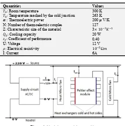
Figure 1 shows a thermoelectric micro-fridge (cooler), having a type Bismuth tellurium type TEC1-12706 module Figure 2 [7, 8] whose characteristics are given in Table 1. It is composed of a fan which extracts the hot air released by the outdoor radiator and an indoor fan that convects cold air into the cooler Figure 3.
Figure 1. Thermoelectric micro-fridge (cooler).
Figure 2. TEC1-12706 Bismuth tellurium type module.
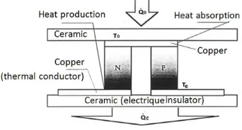
Figure 3. Thermoelectric installation composed of Peltier module.
Table 1. Initial technical characteristics of the installation.
Quantities Values
%&: Room temperature 300 K
% : Temperature reached by the cold junction 263 K
( : Thermoelectric power 200 ) V/K N: Number of thermoelectric couples 127 Z: Characteristic size of the material 3× 10,-.,
: Cooling capacity 20 W
/0: Coefficient of performance 0,40
U: Voltage 12 V
1: Electrical resistivity 10,2Ω3
I: Current 6A
Figure 4. Block diagram of the assembly.
2.2. Method
Figure 5. Peltier thermo-electric system.
1. Heat absorbed or evacued at welding points
On the welding points appears a warmth that is expressed through the relationship:
= 4. . 5 (7) (1)
With:
-π: Peltier coefficient (V);
-I: Intensity of the module supply current (A); -τ: Time in second (s).
2. Heat received as a result of thermal conduction
The material is a thermal conductor; the heat conveyed is expressed by:
9= (: + : )(%;− % )5 (J) (2)
With:
: + : = : = =>? (3)
L: Length of the portion (m);
k: Thermal conductivity constant (W/m2K) λ: Thermal conductibility of the portion (W/K); S: Section (m2)
3. Heat QJ evacuated by half by Joule effect an half the middle
The heat gained by Joule effect and in the environment is expressed by:
@= (A + A ) 5 (7) (4)
With R + A = A = 1?
>: Resistance of a thermocouple
(Ώ)
ρ: Electrical resistivity of the material. (Ώm)
4. Heat taken by the thermoelement in the middle has cool:
In stationary operating regime, the sum , 9, @ of the three components is equal to the heat evacuated by Peltier effect, i.e.:
= + 9+ @ (J) (5)
By replacing (1), (2), (3), (4) in (5) we have:
4. . 5 = + (: + : )(%;− % )5 + (A + A ) 5 (6)
Depending on the time, we have:
=DE = 4 − 0,5(A + A ) − (: + : )G% (7)
Considering: %;= %&
-Ta: Ambient temperature (K);
-T0: Temperature of the cold side of the module (K) -TC: Temperature of the hot side of the module (K) -U= A : Electric power voltage (V);
-∆T = %&− % : Temperature difference between the ambient and the cold side of the module (K);
-k1, k2: Thermal conductivity of the tow materials (W/m2K)
Between the Peltier coefficient and the Seebeck coefficient, there is relationship:
4 = (H − H )% = H% (8) -H , H : Seebeck thermoelectric coefficient of the tow materials (V/K);
We can express the heat absorbed Q0 depending on the U tension by relationship:
=DE = H% − 0,5A − :G% = IH% − 0,5 − : G%J (9)
5. The electric power supply Pe of the module. This power is composed of the following terms:
a. The term Pt represents the component to overcome thermo-electromotor voltage
P"= EI = (α − α )(TO− T )I = (α − α )ΔT. I (Q) (10)
b. The term Pj represents the component of the electro-caloric effect
PR= (R + R )I (Q) (11)
It result in the total electrical power Pe expressed by the relationship:
ST= P"+ PR= URI + αΔTVI = UU + α(TO− T )VI (W) (12)
6. Maximum coefficient of performance
The maximum value of the coefficient of performance
noted εf depends mainly on the optimum value of the current or the supply voltage and the parameters α and Z of the materials used for the semiconductors. Its expression according to the current or the tension is:
ƐY =DZ[= , ,2 ,\^]_
`a(bc,b ) (13)
The optimal voltage Uopt which gives the maximum value
of the coefficient of performance is defined such as:
dƐe
d = 0 (14)
We obtain the second degree equation of U = Uopt, the optimum tension on the form:
kRαY + 2kRY − 0,5α∆T − αT = 0 (15)
i = ∆ (16)
It comes:
i =,\ ,j(\ )k`\ kI `∆lkJ
\ (17)
i =,\ `j(\ )k`\ kI `
∆l kJ
\ (18)
The supply voltage being positive, we will therefore consider the value of i
Taking into account equation (16), we obtain the optimum voltage followed:
= ∆ m `j `
nk o]I `∆lkJp nk
o]I `∆lkJ
(19)
Denoting by:
q =rk ( sℎuvuswxvyzwys zy{x |Y wℎx 3uwxvyu}) (20)
v =\kI% +∆ J = q I% +∆ J (21)
~ = √1 + v (22) The expression of the current corresponding to the maximum coefficient of performance can be written:
=€ =•,∆ x (23)
and the the average temperature as:
%ƒ „ = `n= % +∆ (24)
By reducing the optimal tension in the expression of the coefficient of performance, we obtain:
冇Oˆ=b∆bX
, ,2Š∆ŠˆŒ•‹‹ ,ŠŽ••Š ˆŒ‘‹‹
`Œ•‹‹ (25)
In the expression obtained, we notice the presence of the factor
∆ which represents the coefficient of performance of
the reference Carnot cycle, delimited by the temperatures % and %&.
/;=∆ = ’, (26)
Then (25) becomes:
/0ƒ&“ = /;”1 −•I1 + •,2–J − — ˜×•×•,•` ™ (27)
7. Optimum voltage of a thermocouple
The optimum voltage for a thermoelectric torque is defined by:
= •,×∆ (š) (28)
8. Electrical resistance of a thermocouple.
According to equation (23) this resistance is defined as follows:
A =› ∆
‹ ×(•, ) (Ώ) (29)
9. Total electrical resistance of the module battery It is calculated by:
A =›
‹ (Ώ) (30)
10.Average temperature reached by the module It is determined by:
%ƒ „ = `’= % +∆ (.) (31)
11.Maximum cooling capacity of a thermoelectric couple The maximum cooling capacity of a thermocouple is obtained under optimum conditions where the intensity of the electric current is optimal. By neglecting the heat transmitted by conduction towards the cold welds (Q˙F = 0), and considering the case where k = 0, the equation (1) of the cooling capacity of the module is written:
= H% − ›k= − • (32)
With: Q!= αT I (Term related to the Peltier effect, cold
side), QR=Ÿk (Term related to the Joule effect). The optimum value of the current for which Q0 becomes maximal, is obtained by the relation:
dD
d› = 0 (33)
We have
dD
d› = H% − A (34)
Let the optimum current for which 0 be maximal:
= (35)
With R=R1. Then (40) becomes:
ƒ&“=( )k−( )k (36)
Finally:
ƒ&“= k k(Q) (37)
12.Number of thermoelectric couples under optimal conditions
The number Nopt of thermoelectric couples in optimal conditions is defined by:
=
‹ (38)
Taking into account the number of thermoelectric couples housed in the soles or blocks of the module, this power is obtained by the relation (39):
ƒ&“= × ƒ&“ (W) (39)
14.Intensity of the current for which is maximum The optimal current under the conditions of ƒ&“:
= (A) (40)
15.Maximum temperature difference
Taking into that = 0 and ƐY = 0, we obtain the maximum temperature difference such as:
∆%ƒ&“ = 0,5 × q × % (41)
The minimum temperature of the cold junction under those maximum conditions is defined by:
%ƒ¡¢¡=£ ` ¤’,
¤ (42)
16.Minimum electrical power required by the module. Under the optimization conditions, the electrical power during operation of a Peltier thermoelectric module is not obtained directly by the product U×I, it can be deduced by the relation:
ST=D•e (43)
In this relation (43), the power is minimal for /0= εmax It is defined by the relation:
Sƒ¡¢ =•e—’¥D (44)
17.Intensity of the current for which εf is maximum The intensity of the current which gives the maximum of the cooling efficiency is:
¦Z =Z—§¨ (45)
18.Thermal power discharged by the module
The thermal power discharged by the module is defined by the following relation (46):
; = + Sƒ¡¢ (46)
19.Maximum electrical power consumed by the module The maximum electrical power required by the module depends on the optimum current value corresponding to the maximum cooling capacity. It is determined by:
Sƒ&“= A ∗ ª « + H∆%¬ (47)
20.Intensity of the current of the module power supply. There are two possible choices of supply current, the first choice is the optimal value relative to the maximum coefficient of performance. This current will allow the module to consume minimal electrical power. The second choice is to attribute to the feed current the value of current corresponding to the maximum cooling capacity. This current will provide the module with maximum electrical power. For greater security, the optimum current Iopt supply of the module will be chosen in the interval ; . We will take as a precaution the average value of currents et or:
=›‹ `›k (48)
3. Discussion of Results
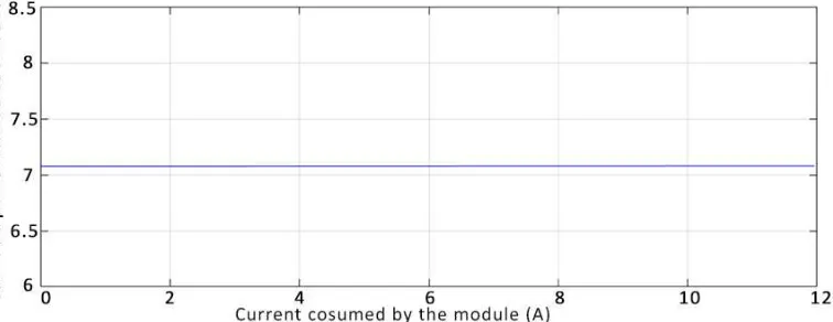
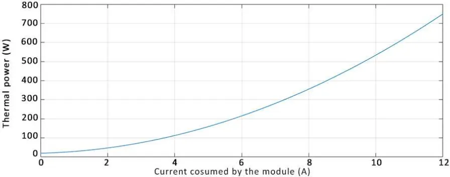
On the graphs, the intensity of the supply current of the module has been represented on the abscissa. The simulation was done at room temperature Ta = 300K. For each variation of the supply current of the module, it is noted that the coefficient of performance of the reference Carnot cycle remains constant Figure 6. While the real coefficient of performance of the minimum electrical power required by the module will be calculated with respect to this first optimal current Figure 7. The minimum electrical power required per module will be calculed in relation to this first optimal current. Figures 8 and 9 show that the electrical and thermal power gradually vary according to the supply current. The cooling power has an arrow which shows the existence of a maximum corresponding to a second optimum value of the module supply current. The maximum value of the electrical power demanded by the module will be calculated as a function of this second optimal current.
a)Coefficient of performance of the Carnot cycle
b)Coefficient of performance of the installation
Figure 7. Variation of the performance coefficient of the installation according to current I.
c)Electrical power of installation
Figure 8. Variation of the electrical power of the installation according to the current I.
d)Heat flow to be evacuated by the module
Figure 9. Heat flow variation versus current I.
Figure 10. Variation of the cooling capacity of the plant as a function of the current I.
On the other hand, the observations made on the graph of the refrigerating power Figure 10, are such that:
At the initial moment, I = 0A, which gives zero cooling capacity, corresponds to the de-energized state of the module. When I∈] 0; Iopt [, The temperature of the cold junction of the module decreases progressively until it reaches the calibration value or its minimum value as a function of the voltage and the supply current. The cooling capacity follows the same progressive rate of change in the increasing direction, since it is related to both the temperature of the cold junction and the supply current of the module. Which is obvious. When the current varies, the cooling capacity also varies.
At I = Iopt, the optimum operating point (Iopt; 0max), is the point where the steady state is established between the cooling effect of Peltier and the heating effect of Joule. The maximum cooling capacity is provided on the cold side and the Joule effect tends to be concealed by the cooling effect of
Peltier. Under these conditions, the flow on the cold side becomes twice the heat flux released by the Joule effect.
For I∈] Iopt; +∞[, the supply current exceeds the optimal
current gradually, the power released by Joule effect gradually increases and a large amount of heat is transmitted gradually by conduction to the cold junction, which reflects the fact that the temperature cold goes back up to tend towards the temperature of the hot welding. Hence the cooling capacity in turn also decreases gradually.
When I → I∞ = 2 × , the heating power released by the Joule effect reaches its extremes, the temperature of the cold part and the temperature of the hot part of the module vary until a maximum temperature difference is reached.. A second steady state is established between the cold side flow and the Joule effect heat flux. Under these conditions, the cooling capacity is canceled again.
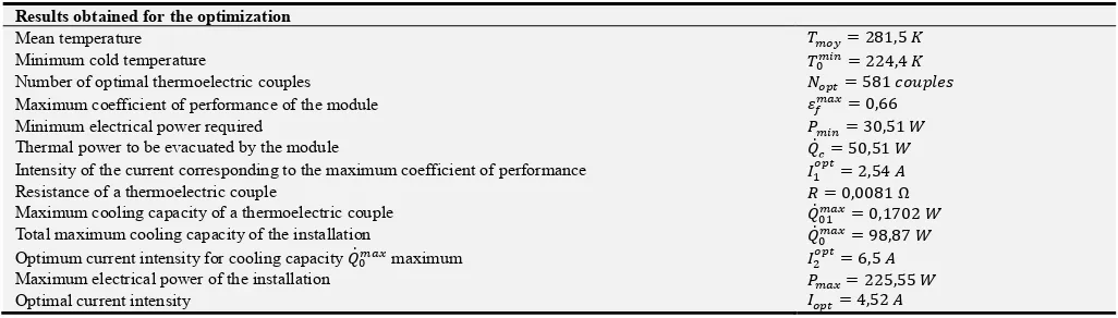
Table 2. Digital application of the optimization of the thermoelectric micro-fridge.
Results obtained for the optimization
Mean temperature %ƒ „= 281,5 .
Minimum cold temperature %ƒ¡¢= 224,4 .
Number of optimal thermoelectric couples = 581 s|°±}xz Maximum coefficient of performance of the module /0ƒ&“= 0,66
Minimum electrical power required Sƒ¡¢= 30,51 Q
Thermal power to be evacuated by the module ;= 50,51 Q Intensity of the current corresponding to the maximum coefficient of performance = 2,54 ´ Resistance of a thermoelectric couple A = 0,0081 Ω Maximum cooling capacity of a thermoelectric couple ƒ&“= 0,1702 Q Total maximum cooling capacity of the installation ƒ&“= 98,87 Q Optimum current intensity for cooling capacity ƒ&“ maximum = 6,5 ´ Maximum electrical power of the installation Sƒ&“= 225,55 Q
Optimal current intensity = 4,52 ´
4. Conclusion
It goes without saying that we always try to obtain a better coefficient of refrigeration performance of an installation while keeping in mind that it can not exceed its theoretical maximum namely the coefficient of performance of Carnot. Due to the compact nature and easy implementation of the Peltier thermoelectric modules, it is necessary to go through an optimization of the main parameters to improve its
performance. One of the objectives of this study was to propose the mathematical model of the Peltier effect, which makes it possible to optimize the coefficient of performance and the cooling capacity of the installation.
that this coefficient of performance is much higher than that presented by the manufacturer:
/0ƒ&“= 0,66 > /0= 0,40, for an optimum intensity much
lower than that prescribed by the manufacturer is: =
4,52 ´ < 6 ´. Finally, to ensure optimum operation of the installation, the regulating system of this one will have to be programmed according to the optimal current.
Nomenclature
I: Intensity of the module supply current
I !": Optimum current intensity corresponding to the maximum coefficient of performance
I !": Optimum current intensity relative to the maximum cooling capacity
I : Intensity of the optimal power supply of the module k: Thermal conductivity constant
N: Number of thermoelectric couples
N : Optimum number of thermoelectric couples
Pƒ¡¢: Minimum electrical power of the installation
Pƒ&“: Maximum electrical power of the installation
PT: Electrical power of the installation
: Cooling capacity of the module
;: Thermal power to be evacuated by the module ƒ&“: Maximum cooling capacity of a thermocouple ƒ&“: Maximum cooling capacity of the installation
: Cold side flux, related to Peltier effect
»: Thermal flux, related to the Joule effect
R: Resistance of a thermocouple
R : Total electrical resistance of the module battery
T&: Ambient temperature
T: Temperature of the cold side of the module
Tƒ¡¢: Temperature of the installation
T‡¼½: Minimum cold temperature of the installation
U: Peltier module power supply
U : Optimum supply voltage of a thermocouple
H: Thermoelectric power or Seebeck coefficient
/0: Coefficient of performance of the installation
/0ƒ&“: Maximum performance coefficient of the installation
∆T: Temperature difference between the ambient and the cold side of the module
∆T‡Oˆ: Temperature difference between the ambient and
the cold side of the module
1: Electrical resistivity of the material.
References
[1] Luis David Palatiño López (2004). Caractérisation des propriétés thermoélectriques des composants en régime harmonique: Technique et Modélisation. Thèse de doctorat, Université de Bordeaux 1, Ecole Doctorale des Sciences Physiques et de l’Ingénieur.
[2] Véronique DA ROS (2008). Transport dans le composés tyhemoélectriques Skutterudites de type A“¾¿À,„ y„Á (R = Nd, Yb et In). Thèse de doctorat, Université de Lorraine, Institut National Polytechnique de Lorraine.
[3] Jean David GRENON (2016). Système de mesure des propriétés thermoélectriques appliqués au phosphore noire. Mémoire, Université de Montréal, Eole Polytechnique de Montréal.
[4] Jean Baptiste VANEY (2014). Contribution à l’étude des propriétés de vitrocéramiques et verres de chalcogénures semi-onducteurs. Thèse de doctorat, Université de Lorraine, Institut Jean Lamour (Nancy)-Institut Charles Gerhard (Montpelier).
[5] Renaud de la Taille-Pierre Courbier (1984). La physique amusante/Science et vie. Collection Savoir et Comprendre. 24 expériences réalisées par Science et vie-Pierron. Pages 6367. [6] Pierre CHAPOUL, Christophe DOM, Paul GALLAIS, Kevin
GUERINEAU, Jean Baptiste MOUSSARD (2008).
Conversion de la chaleur en électricité: Etude du module thermoélectrique à effet Peltier. Rapport du projet de physique, Institut National des Sciences Appliquées de Rouen. Pages 2.
[7] Robert OTEY et Barry MOSKOWITZ (2001). Thermoelectric coolers offer efficient solid-stade heat management options. oe magazine.
[8] J. G. STOCKHOLM (2002). Générateur thermoélectrique, Énergie potable: autonomie et intégration dans l’environnement humain. -Cachan-Journées électrotechniques du club EEA.
[9] Pr. Dr. Ing. Radcenco VSEVOLOD Sef Lucr. Ing. Porneală SAVA Asist. Ing. Alexandru DOBROVICESCU (1983).
Processe in instalatii frigorice. EDITURA DIDACTICĂ PEDAGOGICĂ, BUCURESTI. Pages 359-365.
[10] Pierre CHAPOUL, Christophe DOM, Paul GALLAIS, Kevin GUERINEAU, Jean Baptiste MOUSSARD (2008). Conversion de la chaleur en électricité: Etude du module thermoélectrique à effet Peltier. Rapport du projet de physique, Institut National des Sciences Appliquées de Rouen. Pages 22-23.
[11] Camille FAVAREL (2014). Optimisation de générateurs thermoélectriques pour la production d’électricité. Thèse de doctorat, Université de Pau et des pays de L’Adour, École Doctorale des Sciences Exactes et de leurs Applications. Spécialité: Génie Électrique/Énergétique.
[12] Zhang HY, Mui YC, Tarin M. Analysis of thermoelectric cooler performance high power electronic packages. Appl
Therm Eng (2010); 30: 561–8.
http://dx.doi.org/10.1016/j.applthermaleng.2009.10.020. [13] María Ibañez-Puy, Javier Bermejo-Busto, César
Martín-Gómez, Marina Vidaurre-Arbizu, José Antonio Sacristán-Fernández, Thermoelectric cooling heating unit performance under real conditions Applied Energy 200 (2017) 303–314. http://dx.doi.org/10.1016/j.apenergy.2017.05.020.
[14] Marco Nesarajah and and Georg Frey, Thermoelectric Power Generation: Peltier Element versus Thermoelectric Generator, 978-1-5090-3474-1/16/$31.00 (2016) IEEE. [15] Xiao Zhang, Li-Dong Zhao, Thermoelectric materials: energy
conversion between heat and electricity, Journal of Materiomics (2015), doi: 10.1016/j.jmat.2015.01.001. [16] Zeki Yilmazoglu, Experimental and numerical investigation of
a prototype thermoelectric heating and cooling unit, Energy
and Buildings (2015),
[17] Hamidreza Najafi, Keith A. Woodbury, Optimization of a cooling system based on Peltier effect for photovoltaic cells,
Solar Energy 91 (2013) 152-160.