Comparison of Different methods of Estimation for Transmuted Lomax Distribution

(1)

Comparison of Different methods of Estimation for Transmuted Lomax

Distribution

Rajiv Saksena, Ashok Kumar

*

Department of Statistics, University of Lucknow, Lucknow, India

ABSTRACT

Accurate estimation of parameters of a probability distribution is of massive importance in statistics. Biased and vague estimation of parameters can lead to misleading results. In this paper, we consider the estimation of unknown parameters for the transmuted Lomax distribution. The estimation of parameters will be handled using maximum likelihood estimation, method of moments and L-moments method. A Monte Carlo Simulation is used to make comparison among them.

Keywords: Maximum likelihood estimation, method of moments, L-moments method, Monte Carlo Simulation.

I. INTRODUCTION

The Lomax distribution, also called the Pareto Type II distribution, is a heavy-tail probability distribution often used in business, economics and actuarial modeling. It was used by Lomax (1954) to fit data in business failure. Ashour and Eltehiwy (2013) generalized the Lomax distribution by using transmutation map approach suggested by Shaw and Buckley (2007). This new family of distribution called Transmuted Lomax distribution. According to the Quadratic Rank Transmutation Map (QRTM) approach the cumulative distribution function (cdf) satisfies the relationship

( ) ( ) ( ) ( ) (1) which on differentiation yields,

( ) ( )[( ) ( )] (2)

where ( )nd ( ) are the corresponding probability density functions (pdf) associated with ( ) and ( )

respectively and . Extensive information about the quadratic rank transmutation map is given by Shaw and Buckley (2007). Ashour and Eltehiwy (2013) used the above formulation for a pair of cumulative distribution functions ( ) and ( ) where ( ) is a sub-model of ( ). A random variable X is said to have a transmuted probability distribution function with cdf

 

F x

if

( ) ( ) ( ) ( ) (3) where ( ) is the cdf of the base distribution.

(2)

comparison among the estimation methods. Finally, this study is concluded in Section 5.

II. TRANSMUTED LOMAX DISTRIBUTION

A random variable is said to have a transmuted Lomax distribution with parameters θ, γ and ( ) if its cumulative distribution function is given by

( ) ( )( ( ) ₎ ( ( ) ₎

(4)

and the probability density function of X is given by

(x)= [( ) { ( )_{( )} }] (5) Fig. 1(a) shows the shape of pdf of the transmuted Lomax distribution for few selected values of the parameters.

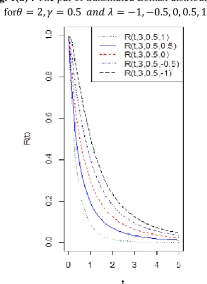
The transmuted Lomax distribution can be useful model to characterize failure time of a given system because of its analytical structure. Reliability is the probability that an item will not fail prior to a specified time t and is defined as ( ) ( ) . The Reliability function of the transmuted Lomax distribution is given by

( ) ( ) ,( )( ( ) _{) ( ( )} ₎ _- ₍₆₎

The reliability function has also known as survival function. The shape of reliability function of the transmuted Lomax distribution for few selected values of the parameters is shown in Fig 1 (b).

The hazard rate function is the conditional probability of failure, given it has survived to the time t and is defined as ( ) ( )_{( )} The hazard rate function for transmuted Lomax distribution is given by

( ) _{( )} [( ) { ( ) }]

[ {[ ( ) _{][( ) { ( )} _}]}] (7)

Fig. 1(a) : The pdf of transmuted Lomax distribution for

Fig. 1(b): Reliability function of transmuted Lomax distribution for

III. PARAMETR ESTIMATION OF

TRANSMUTED LOMAX DISTRIBUTION

(3)

maximum likelihood estimation, method of moments and L-moments.

3.1 MAXIMUM LIKELIHOOD ESTIMATION

Let

x x

₁

, ,...,

₂

x

_n be a random sample of size n from transmuted Lomax distribution. Its likelihood function is given by

∏ [( ) { ( ) }]

∏ ( )( )

(8) The log-likelihood function can be written as

( ) ( ) ∑ [ ] ∑ [( ) { ( ) _}] ₍₉₎

The normal equations become

∑ ( ) ∑ ( ) ( )

[( ) { ( ) _}]

(11)

∑( ) _{( )} ∑ ( ) ( ) [( ) { ( ) _}]

(12)

∑

{ ( ) _}

[( ) { ( ( ) _)}]

(13)

The MLE of can be obtained by solving the nonlinear system of equations (11), (12) and (13) using

=0,

=0 and

=0, respectively.

3.2 METHOD OF MOMENTS

The rth_{moment of a transmuted Lomax random variable} X is given by

( ) ∫ [( ) { ( )_{( )}_{( )} }]

( )∑( ) ( ) ( ( ) ) _∑

( )( ) ( ( ) )

(14)

where, B(. , .) is the beta function defined by B( ) ∫ _{( )}

The first four moments can be obtained by taking r = 1, 2, 3 and 4 in (14) as follows:

( )_{* (}

) + * (

) +

( )_{* (} _{) (} ₎

+ * ( ) +

( )_{* (} _{) (} ₎

( ) +

* ( ) ( )

( ) +

( )_{* (} _{) (} ₎

( ) ( ) +

* ( ) ( )

( ) ( ) +

We can obtain the moment estimator of by using the following equations:

∑

i.e.

( ̂)

̂ * ( ̂ ) + ̂

̂ *( ̂ ) + ̅ (15)

( ̂)

̂ * ( ̂ ) ( ̂ ) + ̂

̂ [ ( ̂ ) ( ̂ )

∑

(16)

( ̂)

̂ * ( ̂ ) ( ̂ )

( _̂ ) + ̂_̂ [ ( _̂ )

( _̂ ) ( _̂ ) ∑

(17)

( ̂)

̂ * ( ̂ ) ( ̂ )

( _̂ ) ( _̂ ) + ̂_̂ [ (

̂ ) ( ̂ ) ( ̂ ) (

̂ )

∑

(18)

We can obtain ̂ ̂ ̂ by solving nonlinear equations (15), (16) and (17) numerically.

3.3 L-MOMENTS METHOD

(4)

in a conceptual random sample of size r

from the underlying population. Here, ( )

which is the same as the population mean.

( ) an alternative to the population standard deviation. Similarly are alternatives to the measure of skewness and kurtosis respectively. L-moments sometimes bring even more efficient parameter estimation of the parametric distribution than those estimated by the maximum likelihood estimation and method of moments for small samples (Hosking (1990), Tomer and Kumar (2014)).

3.3.1 Population L-moments

The population L-moments of order r was given by Hosking (1990) as follows:

∑ ( ) ( ) ( ) (19) where

( ) _{( )} ∑( )( ) ∫ [

( ) _]( ) _{( )} ( ) *( )

{ ( ) _}( )₊

=_{( )} ∑( )( ) [( )* (

( )) _{( )}+ * (

( )) _{( )}+]

(20) Substituting from (20) in (19), the population

L-moments are given as

∑ ( ) ( )( ) ( )

∑ ( )( ) [( )* (

( ))

+

_{* (}

( ))

( )+] (21)

The first three L-moments can be obtained by taking r = 1, 2, 3 in (21) as follows

( )_{* (}

) + * (

) +

( )_{* (} _{) (}

)+ _{* (} _{) (}

)+

( )_{* (} _{) (} ₎

( )+ * ( ) (

) ( )+

3.3.2 Sample L-moments

The sample L-moments was given by Elamir and Seheult (2003) and defined as.

∑ ∑ ( ) ( )( )( )

( )

L-moments estimator for can be obtained as follows:

,

1, 2,3

r r

L



l

r



We get,

( )

* ( ) + * ( )

+ ̅

(22)

( )_{* (} _{) (}

)+

* ( ) ( )+

_{( )}∑( ) ̅ (23)

( )_{* (} _{) (} ₎

( )+

* ( ) (

)+ ∑( )( ) ( )( ) ( )( )_{( )( )}

(24)

IV. MONTE CARLO SIMULATION STUDY

In this section, a Monte Carlo simulation study is conducted to compare estimators obtained from maximum likelihood estimation, method of moments and L-moment method for the transmuted Lomax distribution. This comparison is based on mean square errors (MSEs). Here, we have used R i386 3.4.0 software for simulation study. We generated the samples of sizes 30 (20) 110 and computed mean square error

(MSE) of the estimates of unknown

(5)

results for MSEs using different methods of estimation are listed in Table 1.

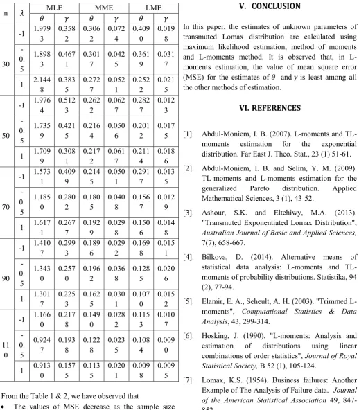
Table 1: The values of MSE for different methods of estimation

n MLE MME LME

30

-1 1.979 3 0.358 2 0.306 2 0.072 4 0.409 0 0.019 8 -0. 5 1.898 3 0.467 1 0.301 7 0.042 5 0.361 9 0.031 7

1 2.144 8 0.383 5 0.272 7 0.052 1 0.252 2 0.021 5 50

-1 1.976 4 0.512 3 0.262 2 0.062 7 0.282 7 0.012 3 -0. 5 1.735 9 0.421 5 0.216 4 0.050 6 0.201 2 0.017 5

1 1.709 9 0.308 1 0.217 2 0.061 7 0.211 4 0.018 6 70

-1 1.573 1 0.409 9 0.214 5 0.050 1 0.291 7 0.013 5 -0. 5 1.185 0 0.280 2 0.180 5 0.040 8 0.156 7 0.012 9

1 1.617 1 0.267 7 0.192 9 0.029 8 0.150 6 0.014 8 90

-1 1.410 7 0.299 3 0.189 6 0.029 2 0.169 8 0.015 1 -0. 5 1.343 0 0.257 0 0.196 2 0.036 8 0.128 5 0.020 6

1 1.301 7 0.225 3 0.162 5 0.030 1 0.107 0 0.015 2 11 0

-1 1.166 0 0.217 8 0.149 0 0.028 2 0.115 3 0.010 7 -0. 5 0.924 7 0.193 8 0.122 8 0.023 5 0.108 4 0.009 0

1 0.913 0 0.157 5 0.113 5 0.020 1 0.009 8 0.009 5

From the Table 1 & 2, we have observed that

 The values of MSE decrease as the sample size increases.

 For the parameter , we can note that the LME is the best method.

 For the parameter , we can see that the LME is also the best method.

V. CONCLUSION

In this paper, the estimates of unknown parameters of transmuted Lomax distribution are calculated using maximum likelihood estimation, method of moments and moments method. It is observed that, in L-moments estimation, the value of mean square error (MSE) for the estimates of and is least among all the other methods of estimation.

VI. REFERENCES

[1]. Abdul-Moniem, I. B. (2007). L-moments and TL-moments estimation for the exponential distribution. Far East J. Theo. Stat., 23 (1) 51-61.

[2]. Abdul-Moniem, I. B. and Selim, Y. M. (2009). TL-moments and L-moments estimation for the generalized Pareto distribution. Applied Mathematical Sciences, 3 (1), 43-52.

[3]. Ashour, S.K. and Eltehiwy, M.A. (2013). "Transmuted Exponentiated Lomax Distribution",

Australian Journal of Basic and Applied Sciences,

7(7), 658-667.

[4]. Bilkova, D. (2014). Alternative means of statistical data analysis: L-moments and TL-moments of probability distributions. Statistika, 94 (2), 77-94.

[5]. Elamir, E. A., Seheult, A. H. (2003). "Trimmed L-moments", Computational Statistics & Data

Analysis, 43, 299-314.

[6]. Hosking, J. (1990). "L-moments: Analysis and estimation of distributions using linear combinations of order statistics", Journal of Royal

Statistical Society, B 52 (1), 105-124.

[7]. Lomax, K.S. (1954). Business failures: Another Example of The Analysis of Failure data. Journal

of the American Statistical Association 49,

(6)

[8]. R Core Team (2017). R: A language and environment for statistical computing. R Foundation for Statistical Computing, Vienna, Austria. URL https://www.R-project.org/.

[9]. Shaw, W. and I. Buckley (2007). The Alchemy of Probability Distributions: Beyond Gram-Charlier Expansions, and a Skew-Kurtotic-Normal Distribution From a Rank Transmutation Map. Research report.