www.nat-hazards-earth-syst-sci.net/8/671/2008/ © Author(s) 2008. This work is distributed under the Creative Commons Attribution 3.0 License.
and Earth
System Sciences
A new computational method based on the minimum lithostatic
deviation (MLD) principle to analyse slope stability in the frame of
the 2-D limit-equilibrium theory
S. Tinti and A. Manucci
Universit`a degli Studi di Bologna, Dipartimento di Fisica, Settore di Geofisica, Viale Berti Pichat, 8 – 40127 Bologna, Italy Received: 18 January 2008 – Revised: 2 June 2008 – Accepted: 4 June 2008 – Published: 16 July 2008
Abstract. The stability of a slope is studied by applying the principle of the minimum lithostatic deviation (MLD) to the limit-equilibrium method, that was introduced in a pre-vious paper (Tinti and Manucci, 2006; hereafter quoted as TM2006). The principle states that the factor of safetyF of a slope is the value that minimises the lithostatic deviation, that is defined as the ratio of the average inter-slice force to the average weight of the slice. In this paper we continue the work of TM2006 and propose a new computational method to solve the problem. The basic equations of equilibrium for a 2-D vertical cross section of the mass are deduced and then discretised, which results in cutting the cross section into ver-tical slices. The unknowns of the problem are functions (or vectors in the discrete system) associated with the internal forces acting on the slice, namely the horizontal forceEand the vertical forceX, with the internal torqueAand with the pressure on the bottom surface of the slideP. All traditional limit-equilibrium methods make very constraining assump-tions on the shape ofX with the goal to find only one so-lution. In the light of the MLD, the strategy is wrong since it can be said that they find only one point in the search-ing space, which could provide a bad approximation to the MLD. The computational method we propose in the paper transforms the problem into a set of linear algebraic equa-tions, that are in the form of a block matrix acting on a block vector, a form that is quite suitable to introduce constraints on the shape ofX, but also alternatively on the shape of E or on the shape ofA. We test the new formulation by ap-plying it to the same cases treated in TM2006 whereXwas expanded in a three-term sine series. Further, we make dif-ferent assumptions by taking a three-term cosine expansion corrected by the local weight forX, or forE or forA, and find the corresponding MLDs. In the illustrative applications
Correspondence to: S. Tinti
given in this paper, we find that the safety factors associated with the MLD resulting from our computations may differ by some percent from the ones computed with the traditional limit-equilibrium methods.
1 Introduction
Determining the stability of a slope is a problem of great interest since a long time to assess the hazard and miti-gate the risk of an area. Different methods of analysis have been developed, ranging from approximated 1-D or 2-D ap-proaches to fully 3-D methods solving visco-plastic equa-tions through finite-element or finite-difference techniques. Usually more sophisticated methods such as 3-D need a very detailed knowledge of the soil and subsoil conditions that are difficult and expensive to acquire, which makes the recourse to simplified techniques often more convenient and more practical to use. The classical limit-equilibrium methods be-long to the category of approximated methods. The meth-ods were firstly introduced with the Fellenius formula (1927) and lately developed by Bishop (1955), by Morgenstern and Price (1965), by Spencer (1967), by Janbu (1968) and oth-ers. They were the starting point of the slope stability anal-ysis and were successfully applied and repeatedly refined, since they are still subject of active research (e.g. Duncan and Wright, 1980; Chen and Morgenstern, 1983; Leschchinsky and Huang, 1992; Chen et al., 2001; Zhu et al., 2003; Jiang and Yamagami, 2004; Karaulov, 2005; Tinti and Manucci, 2006, hereafter quoted as TM2006; Zheng et al. 2007; Pink, 2007).
E
X X
E w
P S
k Water Level
D
z1 z2
x
begx
endy a
b
zw
x z
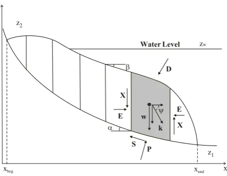
Fig. 1. Sketch of the vertical cross-section of the sliding body cut into slices. Cartesian coordinatesxandzare taken to increase right-ward and upright-ward, as usual. The forces, described in the text, act on each slice. In the discretised version of the analytical problem, slices are defined as the portions of the body comprised between the vertical planesxi−1x/2 andxi+1x/2 The seismic load is a force proportional to the weight of the slice and forms the angleψ
with the horizontal. The loadDis a pressure acting on the body top surface.
by all balance equations the number of unknowns (i.e. the safety factor and the component of the forces and torques acting on the slices) is greater than the number of equations with the consequence that the solution, and therefore even the computed safety factor, is not unique. This is usually overcome by means of ad-hoc assumptions (constraints), that differ from one author to the other, and the correspondent re-sulting safety factors may depart by 5–10% from one another. In a previous paper (TM2006) we have called the attention on this issue and we have proposed a drastic change of view for the limit-equilibrium approach. The factor of safety, instead of an unknown, was proposed to be treated as a known pa-rameter, sayF∗, that is left to range within a given interval. For each value ofF∗, a solution, sayS(F∗), to the equilib-rium equations is computed. The unique solution to the prob-lem is found by introducing and applying a new criterion, that was called the “Principle of Minimum Lithostatic Devi-ation (MLD)”. The lithostatic deviDevi-ationδ expresses the ra-tio of the average magnitude of the internal slice-slice forces and the total weight of the sliding mass (see formula (18) of TM2006). The MLD principle means that one calculates the value ofδ for each computed solutionS(F∗), obtaining the relationδ(S(F∗))or more simplyδ(F∗), and, eventually one selects the safety factor F corresponding to the minimum value ofδ, i.e.F=F∗(δmin). In the present paper the valid-ity of the MLD criterion is confirmed, but the computational technique used to solve the set of the equilibrium equations, i.e. to obtain the solutionS(F∗), is revisited and a procedure based on matrix calculus is introduced that is faster and
eas-ier to manipulate than the method previously used and may be easily extended to handle limit-equilibrium analyses for bodies sliding on surfaces (3-D) rather than along profiles (2-D).
2 Formulation of the problem
The stability of a body in 2-D is studied by taking into ac-count vertical cross-sections. The section belongs to the plane(x, z)and both, the body and the slope, are assumed to be uniform along the horizontal axis y. In the sketch of Fig. 1 a vertical section is given where the body is con-fined between the sliding surfacez1(x)and the upper surface z2(x). In limit-equilibrium analysis the section is subdivided into vertical slices and the governing system of equations is obtained by imposing the balance of all forces and torques acting on these slices.
2.1 The set of equilibrium equations
We use the same formalism we adopted in TM2006 where the reader may find a detailed derivation of the basic set of equations. Here we limit to recall the notions essential to understand the subsequent analysis. Forces are depicted in Fig. 1:w(x)is the slice weight per unit area,D(x)is an ex-ternal pressure acting on the upper slide surface,P (x) and S(x)are respectively the pressure and the shear stress at the base of the slice,E(x)andX(x)are the horizontal and ver-tical components of the inter-slice forces, whileA(x)is the component of the torque along the axisy. They are functions of the horizontal coordinatex, and each slice is taken to have an infinitesimal width1x, a finite heightz2(x)−z1(x)and to be comprised betweenx−1/21xandx+1/21x.
The set of equilibrium equations may be given the follow-ing expression (see TM2006):
d
dxE+Ptanα−S−Dtanβ= −wkcosψ (1) d
dxX+P +Stanα−D=(1+ksinψ ) w (2) d
dxA−z1 d
dxE−X−Dtanβ (z2−z1)=−wkcosψ (zB−z1) (3)
F S= ¯c∗+Ptanφ¯0 (4)
with
¯
c∗= ¯c0−utanφ¯0
the basal surface. According to the Mohr-Coulomb law,Smax is given by:
Smax(x)= ¯c0(x)+(P (x)−u(x))tanφ¯0(x)
where u(x) is the pore pressure dependent on the piezo-metric level, andc¯0andφ¯0 are average values of the mate-rial cohesion and of the friction angle, as better explained in Sect. 2.2. Consistently with this view, Eq. (4) imposes that shear strength and stress are proportional via the coefficient F, the safety factor, and that F may be used to mark the boundary between stable (F >1) and unstabe (F <1) regions. In Eqs. (1)–(3)α (x)andβ (x)are the angle of slope re-spectively at the base and at the top of the slice. The slice weightwis defined as:
w(x)=g z2
Z
z1
ρ(x, z)dz
whereρis the density that depends on the position (x, z)in heterogeneous bodies.
The torqueA(x)is computed with respect to the centre of mass of the slidezB(x)which is given by:
zB(x)= z2
R
z1
ρ (x, z) zdz
w(x)
The loadD(x)on the upper surface, when it is due to water as in the case of a body that is totally or partially submerged, can be expressed as follows:
D(x)=ρwg[zw−z2(x)] z2(x) < zw D(x)=0 z2(x)≥zw
wherezwis the water level andρwthe water density.
Equations (1)–(3) account also for the seismic load, which is assumed to act at the centre of mass of the slice along the directionψand to be proportional to the slice weight through the coefficientk.
The set of Eqs. (1)–(4) is the basic system for the slope stability problem according to the limit-equilibrium method. It has to be complemented by the boundary conditions, stat-ing that all the inter-slice forces and torques vanish at the beginning and at the end of the sliding body:
E(xbeg)=E(xend)=0 (5)
X(xbeg)=X(xend)=0 (6)
A(xbeg)=A(xend)=0 (7)
Equations (1)–(7) form a set of three first-order ordinary dif-ferential equations completed by the corresponding bound-ary conditions and by an additional relationship, Eq. (4). This set contemplates one unknown parameter,F, and five unknown functions defined in the finite domainxbeg, xend
,
namely the basal stresses P (x) and S(x) and forces and torques associated with slice interaction E(x), X(x) and A(x). In this formulation, the sliding surface described by the function z1(x) is considered to be known a priori: it may be circular, as it is assumed in some classical limit-equilibrium methods, or have a more general shape (see Gra-ham, 1984).
2.2 The stratified soil
Assuming a homogeneous sliding body is often an oversim-plification of the problem and may lead to questionable con-clusions on slope stability, especially if there is evidence of the existence of weak layers at some depth. Accounting for a stratified soil in the formulation given in Sect. 2.1 is straightforward. Let us suppose that the body cross-section is composed ofMlayers with layerilying between interfaces i and i+1, and with interfaces described by the functions zint,i(x)andzint,i+1(x)(zint,i < zint,i+1). We can further suppose that the body basez1and topz2coincide with sur-faceszint,1(x)andzint,M+1(x). Material properties such as densityρ, cohesionc0and friction angleφ0will change from one layer to the next, but incorporating the depth-dependence in the stability equations is quite easy. The expression for the weightw(x)in the previous section is still valid and the in-tegral will reduce to a summation across all layers of the ma-terial columnx (that is formed at most byMlayers). As for cohesion and friction angle, it is remarked that only the val-ues they assume on the sliding surfacez1(x)are of relevance in Eq. (4), i.e. the valuesc0(x, z1(x)) φ0(x, z1(x)). Practi-cally, since the set of Eqs. (1)–(4) cannot be solved analyt-ically, but through numerical methods, it is anticipated here that covering the computational domain
xbeg, xendwith a finite grid with N+1 nodes, implies the partition of the body cross-section into N vertical slices. Such a discretization im-plies further that, given the slice corresponding to the interval
xi, xi+1, in place of local values of cohesion and of friction angle, average valuesc¯0andφ¯0 are to be used, with average computed over the base of the slide, according to the formu-las:
¯
c0i= xi+1
R
xi
c0(x, z1(x)) dx
xi+1−xi
¯
φ0i= xi+1
R
xi
φ0(x, z1(x)) dx
xi+1−xi
2.3 The traditional methods
Traditional methods of limit equilibrium treat the safety fac-tor as an unknown parameter. The solution to the set of Eqs. (1)–(7) is underdetermined since there are four equa-tions for five unknown funcequa-tions ofx and for one unknown parameter,F. Despite the existence of more than one solu-tion, the first methods were devised in times when numerical computing was still a very hard job and introduced drastic simplification to allow the computation of at least one so-lution. Fellenius (1927) assumed that inter-slice forces are null; Bishop (1955) and Janbu (1968) posed vertical forcesX equal to zero and disregarded the horizontal and the vertical equilibrium equations, respectively. On the other hand, Mor-genstern and Price (1965) and Spencer (1967) were the first who tackled the non-uniqueness problem and overcame it by imposing a relationship between the vertical and horizontal components of the inter-slice forces, which is equivalent to add a new equation to the original set (1)–(7). Spencer’s method is taken in this article as representative of classical methods and against it we will compare our results.
3 Determination of the unique solution
The non-uniqueness of the solution has the consequence that also the safety factorF, that is one of the unknowns of the problem, cannot be determined univocally. It can be shown that usually one can find exact solutions to the Eqs. (1)– (7) with very different values ofF, ranging from below to above the critical value of 1. And this in principle is a rele-vant theoretical weakness of this approach, undermining the meaning itself of the analysis. In practice, the additional hy-potheses introduced by Morgenstern and Price, by Spencer and by others, restrict the interval of variability of the safety factor to more acceptable limits. In TM2006 a totally differ-ent approach was suggested, converting the limit-equilibrium method to a minimization problem, whereF is treated as a free parameter, and not as an unknown. Within a given inter-val ofF, say [Fmin, Fmax], one searches the solution to the set of Eqs. (1)–(7) that minimizes the lithostatic deviationδ, and the value of the parameterF corresponding to the minimum value ofδis taken as the final result of the limit-equilibrium analysis. The lithostatic deviation is defined as:
δ=W−1
1 (xend−xbeg)
xend
Z
xbeg
(E(x)2+X(x)2)dx
1/2
where:
W = 1
xend−xbeg xend
Z
xbeg
w(x)dx
Notice thatδis the dimensionless ratio of the average mag-nitude of the internal forces to the total weightWof the
slid-ing mass. Notice further that the conditionδ=0 trivially im-plies that bothE(x)andX(x)are identically zero over the domain
xbeg, xendwhich is a state of equilibrium only for the special case of a body of uniform thickness lying over a uniform slope.
4 Finding the solution
4.1 The discretization
The system of Eqs. (1)–(7) can be set in a more adequate form. In first place, we note that Eq. (4) involves the known parameterF, the known material properties (c¯0,φ¯0andu)and two unknown functionsP (x)andS(x). Hence, with the aid of Eq. (4) one can express S(x)in terms of P (x), and re-place it in all Eqs. (1)–(3). After some manipulations one obtains the following system of equations in the unknown E(x),X(x),A(x)andP (x):
dE
dx +P αE=βE
dX
dx +P αX=βX (8)
dA
dx +P αA−X=βA
including coefficients that are given by: αE=tanα−tan
¯
φ0 F βE=c¯
∗
F +Dtanβ−kcosψ w αX=1+tanαtan
¯
φ0 F βX=D−c¯
∗
F tanα+(1+ksinψ ) w αA=z1αE
βA=Dtanβ (z2−z1)−kcosψ (zB−z1) w+z1βE
(9)
Observe that all such coefficients are known functions of the problem, since they depend on the geometry of the body, on its material properties, on the external loads (water layer and seismic forcing) and on the parameterF. Observe further that some coefficients, such asαEandαX, are dimensionless,
while others are not:αAis a length,βEandβXare pressures,
whileβAis a pressure times a length.
The solution is searched for by numerical means. The computational domain
xbeg, xendis discretised intoNequal intervals of length 1x through the nodal points xi, i ∈
Table 1. Comparison of stability analysis results obtained with the traditional Spencer method, the Tinti and Manucci (T&M) method and with the various applications of the new computational method presented in this paper. The slope is the same as in TM2006. Case 1: no seismic and no water load. Case 2: water load only. Case 3: seismic load only. The best results (i.e. the MLDs) are found in the cells with bold characters. All are in the same raw, since are obtained with the same method.
Method Case 1 Case2 Case 3
F δ F δ F δ
Spencer 1.468 0.1052 1.579 0.1163 0.984 0.1780 T&M 1.409 0.0772 1.510 0.0845 0.925 0.1193 T&M-new 1.409 0.0776 1.509 0.0847 0.926 0.1199 T&M-Xsin 1.409 0.0776 1.509 0.0847 0.926 0.1199 T&M-Xcos 1.405 0.0762 1.505 0.0835 0.920 0.1147
T&M-Ecos 1.415 0.0836 1.510 0.0891 0.922 0.1305 T&M-Acos 1.412 0.0812 1.522 0.0885 0.937 0.1301
p, with pi=p(xi−1x/2), i ∈ [1, N], and in an
analo-gous way the vectorbEwithbE,i=βE(xi−1x/2), the
vec-torbX withbX,i=βX(xi −1x/2) and the vectorbA with
bA,i=βA(xi−1x/2). Similar discretization holds for the
co-efficientαE, but, as will be seen later, instead of a vector it is
more adequate to introduce a diagonalN×Nmatrix AEwith (AE)i,i=αE(xi −1x/2). Analogously we define the
matri-ces AX and AA. We may also introduce (N+1)-component
vectors for forces and torque, but, since these are null at the boundaries in force of conditions (5)–(7), we are allowed to restrict the attention to the internal nodes of the domain. Hence, the unknown functionE(x)is transformed into the (N-1)-component vectore withei=E(xi), i ∈ [1, N−1],
and the same applies to vectorsXanda, i.e.Xi=X(xi)and ai=A(xi). In terms of these discretized quantities, it is easy
to transform the first of the differential Eq. (8), namely the one concerning the equilibrium of the slices along the hori-zontal axis, into the following system of algebraic equations:
e1+p1αE,11x=βE,11x ...
ei− ei−1+piαE,i1x=βE,i1x ....
eN−1−eN−2+PN−1αE,N−11x =βE,N−11x
−eN−1+pNαE,N1x=βE,N1x
(10)
After introducing the rectangularN×(N-1) matrix0 given by:
0=
1 0 0 0 0
−1 1 0 0 0 0 −1 1 0 0 ... ... ... ... ... 0 0 0 −1 1 0 0 0 0 −1
0
C
10 20 30 40 50 60 70 80 90 100
10 20 30 40 50 60 70
z
x
Distance (m)
Height (m)
xi xf
Water level
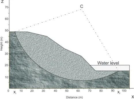
Fig. 2. Vertical cross-section of the body already analysed in
TM2006. The sliding mass is in light grey. The sliding surface has a circular profile centred in C. The soil parametersc0,φ0andρ
are constant, with respective values of 6 kPa, 25◦and 25 kNm−3. The sliding body is partially submerged by a 5 m deep water layer.
the system (10) can be written in the following vectorial form:
0e+AEp1x=bE1x (11)
Analogously, on discretizing the vertical equilibrium Eq. (2) and accounting for the corresponding boundary condi-tion (6), we obtain:
0x+AXp1x =bX1x (12)
In the torque equilibrium Eq. (3), the termXhas to be eval-uated at the interval mid-points, which is obtained by taking the average value between two adjacent nodes. Bearing this in mind and the boundary condition (7), the followingN-1 relations can be obtained:
0a+AAp1x−X1x =bA1x (13)
where use is made of the rectangularN×(N-1) matrix de-fined as:
=1
2
1 0 0 0 0 1 1 0 0 0 0 1 1 0 0 ... ... ... ... ... 0 0 0 1 1 0 0 0 0 1
0 20 40 60 80 100 -20
-10 0 10 20 30 40 50 60
70 T&M
T&M-new T&M Xsin T&M Xcos T&M Ecos T&M Acos
A
(M
N
m
-1 )
Horizontal distance (m)
0 20 40 60 80 100
-5 -4 -3 -2 -1 0 1 2
E
(M
N
m
-1 )
Horizontal distance (m)
T&M T&M-new T&M Xsin T&M Xcos T&M Ecos T&M Acos
0 20 40 60 80 100
-3 -2 -1 0 1 2 3 4 5
X
(M
N
m
-1 )
Horizontal distance (m)
T&M T&M-new T&M Xsin T&M Xcos T&M Ecos T&M Acos
0 20 40 60 80 100
-500 0 500 1000
P
(k
Pa
)
Horizontal distance (m)
T&M T&M-new T&M Xsin T&M Xcos T&M Ecos T&M Acos
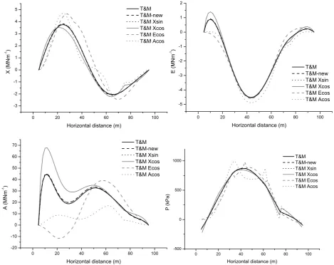
Fig. 3. Graphs of the inter-slice forcesEandX, of the torqueAand of the bottom pressureP corresponding to the best solutions of the
various methods applied for Case 1.
4.2 Non uniqueness of the solution
In order to reduce the degree of freedom of the algebraic sys-tem (11)–(13), some assumptions must be made on the un-knowns. In this paper we will consider restricting hypothe-ses on the form of the inter-slice forcesE andX, and of the torqueA. Consistently with classical limit-equilibrium methods, our first assumption regards the vertical forcesX. Let us expand the functionX(x)over a basis of analytical known functionsfk(x)(for example, a Fourier series
expan-sion), that is truncated to the firstmterms. Correspondingly, the discretised version of such expansion yields the following set ofN-1 equations:
X1= m
X
k=1
vkfk(x1)
X2= m
X
k=1
vkfk(x2) (14)
XN−1= m
X
k=1
vkfk(xN−1)
this can be seen as a mapping of theN-1 unknownsXinto themunknownsv, i.e. the coefficients of the truncated ex-pansion. Formally, after definingfik=fk(xi), the above
re-lations can be synthesised as:
Xi= m
X
k=1
fikνk (15)
0 10 20 30 40 50 60 70 80 90 100 10 20 30 40 50 60 70 z x Meters Meters
xi xf
Layer 1
Layer 2
Layer 3
Fig. 4. Vertical cross-section of the three-layer sliding mass. The soil parameters are given in the text and in caption of Table 2.
free parameters. We can therefore make this distinction ex-plicit by writing:
Xi=fi1ν1+fi2ν2+ m−2
X
k=1
gikqk (16)
where the two unknowns arev1 andv2, and the known pa-rameters and related functions are denoted respectivelyqk
andgikfor sake of clarity.
After introducing the 2-component vectorvand the (m -2)-component vectorqdefined by:
v= v1 v2 q= q1 ... qm−2
as well as the (N-1)×2 matrix F1 and the (N-1)×(m-2) F2
defined as:
F1=
f1,1 f1,2 f2,1 f2,2 fN−1,1fN−1,2
F2=
g1,1 g1,2 ... g1,m−2 g2,1 g2,2 ... g2,m−2 gN−1,1gN−1,2... gN−1,m−2
Equations (16) can be written in this simple vectorial form:
X−F1v=F2q (17)
4.3 Solving the problem
The final algebraic system of equations can be assembled by putting together the above Eqs. (11)–(13) and (17), which leads to:
0e+AEp1x=bE1x 0X+AXp1x=bX1x
0a+AAp1x−X1x=bA1x X−F1v=F2q
(18)
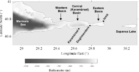
Fig. 5. The Izmit Gulf with its basins in the Maramara sea.
Deˇgirmendere is located in the south-eastern coast close to the end of the Karam¨ursel Basin.
where the unknown vectors e, X, a and v are on the l.h.s. of the system, while vectors on the r.h.s. are known quantities. It is then easy to build a block matrix together with the cor-responding block vectors in the form:
0 0 0 AE 0
0 0 0 AX 0
0 −1x 0 AA 0
0 I 0 0 −F1
e X a p1x v =
bE1x
bX1x
bA1x
F2q
(19)
which is a system of 4N-1 linear equations in 4N-1 un-knowns and very suitable for inversion.
4.4 Hypotheses on the unknown functions and related con-siderations
The form (19) of the problem is quite flexible and allows one to easily explore different assumptions on the shape of the inter-slice forceX(x). In a first instance we assume a trun-cated three-term sine Fourier expansion for X (i.e. we as-sumem=3), which is the same expression we already used in TM2006, where however we computed the solution through a less general ad-hoc method. More specifically we assume that
X(x)=
3
X
k=1 λksin
kπ x−xbeg xend−xbeg
and make the choice thatλ1is a known parameter, whileλ2 andλ3 are unknown quantities. Notice that the above po-sition ensures thatX(x) vanishes at the end points of the domain as required by the condition (6). According to our notation we can write:
gi,1=sin
π i N
i=1,2, .· · ·, N−1
fi,1=sin
2π i N
i=1,2, .· · ·, N−1
fi,2=sin
3π i N
Table 2. Results for stratified soils obtained with all the methods used here. The three-layer stratification is shown in Fig. 4. The ho-mogeneous case is case 1 of Table 1 (γ0=25 kN/m3,c0=6 kPa,φ0=25◦). Case 4 is heterogeneous in density (γ10=22 kN/m3,γ20=28 kN/m3,
γ30=30 kN/m3). Case 5 is heterogeneous in cohesion (c10=6 kPA,c02=100 kPa,c03=200 kPA). Case 6 is heterogeneous as regards the friction angles (φ01=10◦,φ20=15◦,φ30=35◦). Cells with the MLD values have bold characters.
Method Case 1 Case 4 Case 5 Case 6
F δ F δ F δ F δ
Spencer 1.468 0.1052 1.523 0.1034 2.651 0.1164 2.012 0.1136 T&M 1.409 0.0772 1.463 0.0760 2.588 0.0863 2.066 0.0771 T&M-new 1.409 0.0776 1.463 0.0763 2.585 0.0864 2.060 0.0776 T&M-Xsin 1.409 0.0776 1.463 0.0763 2.585 0.0864 2.060 0.0776 T&M-Xcos 1.405 0.0762 1.460 0.0754 2.585 0.0858 2.070 0.0764 T&M-Ecos 1.415 0.0836 1.471 0.0801 2.590 0.0895 2.100 0.0881 T&M-Acos 1.412 0.0812 1.478 0.0803 2.600 0.0898 2.090 0.0823
and identifyλ1withq=q1andλ2andλ3withv1andv2 re-spectively. Inversion of the system (19) provides a solution for any given choice of the known parameters, that are F andq1 in this case. In agreement with the adopted princi-ple of MLD, the solving procedure consists (i) in solving the system (19) by letting these parameters to vary within reason-able intervalsIFandIqthat are obviously spanned at discrete
steps, (ii) in computing the lithostatic deviation correspond-ing to each solution, i.e. in computcorrespond-ingδ (F, q1)within the 2-D spaceIF×Iq, which can be called the searching space,
and eventually (iii) in finding the point in such a space where δtakes its minimum value. The corresponding value ofF is the searched value of the safety factor. It is worth stressing here once more the difference between the traditional meth-ods of limit-equilibrium theory and ours. Those methmeth-ods find only one solution of the equilibrium equations and take the corresponding value ofF as the safety factor of the slope. But we know that a solution can be found for any point of the searching space. Therefore, since the intervalIF may be
shown to include the discriminant value of unity, the conse-quence is that one has no means to judge on the stability of a slope, unless one invokes an additional criterion, such as the MLD principle.
In Table 1 we show the results of our computations applied to the body sketched in Fig. 2, which is the same body the reader can find in TM2006. These results, that will be des-ignated by T&M-new, are compared with the one that were obtained in TM2006 and that are here denoted by TM. As expected, they practically coincide and the slight differences are uniquely due to small numerical rounding errors associ-ated with the fact that in TM2006 we solve the same basic set of equations by using an ad-hoc semi-analytical method, while here we invert system (19) by a standard numerical real-matrix inversion routine.
Since, given a series expansion, one can choose freely the two terms of the series whose coefficients are unknown, we explore the effect of a different choice. In the following we
still make recourse to the three-term sine Fourier expansion, but we take:
gi,1=sin
3π i N
i=1,2, .· · ·, N−1 and
fi,1=sin
π i N
i=1,2, .· · ·, N−1
fi,2=sin
2π i N
i=1,2, .· · ·, N−1
The corresponding solutions will be denoted by T&M-Xsin in this paper. A further explored hypothesis is to consider a different set of base functionsgandf. Instead of sine func-tions, we can take cosine functions multiplied by the local normalised weight to ensure fulfilment of the boundary con-dition (6), i.e. we assume:
gi,1= w(xi)
wmax
cos 2π i
N i=1,2, .· · ·, N−1 (20) and
fi,1= w(xi)
wmax
i=1,2, .· · ·, N−1 (21)
fi,2= w(xi)
wmax cosπ
i
N
i=1,2, .· · ·, N−1 (22)
Herewmaxis defined as the max{w(xi)}i=1,2, .· · ·,N-1.
system of equations can be written in the following “block” forms:
0 0 0 AE 0
0 0 0 AX 0
0 −1x 0 AA 0
I 0 0 0 −F1
e X a
p1x
v
=
bE1x
bX1x
bA1x
F2q
(23)
0 0 0 AE 0
0 0 0 AX 0
0 −1x 0 AA 0
0 0 0 I −F1
e X a
p1x
v
=
bE1x
bX1x
bA1x
F2q
(24)
We have made experiments of both types. In particular, we have selected the three-term expansion given by the co-sine functions (20)–(22) and inverted the system (23) when the position regarded the horizontal forcesE(x), while we have inverted the system (24) when the position regarded the torqueA(x). The results will be referred as T&M-Ecos in the first case and as T&M-Acos in the second.
The formulation of the limit-equilibrium problem pro-posed here leads to the inversion of the “block” system of equations in one of the three forms (19), (23) and (24). We stress that this is a relevant improvement on previous meth-ods: not only on the traditional methods, but also on the TM2006 formulation, since the present version combines the advantage of being computationally fast (as most of the other methods) with a great flexibility, since it allows one to ex-plore quite easily different assumptions on the shape of the unknown functions.
It is relevant also to point out that each hypothesis leads to a different solution for the safety factorF, since this is obtained by minimising the lithostatic deviationδwithin the searching space. In the general case of anm-term expansion like the position (16) the searching space will have dimen-sionm-1, since the involved parameters are them-2 vectorq
andF. The fact that we have a multiplicity of results forF is not crucial since we may resolve such an apparent ambi-guity by making recourse once more to the MLD principle. Indeed we will select as the best solution forF, the one that is associated with lowest value ofδ. This means that there
is no way to judge the goodness of a hypothesis of type (16) a priori. Each of these can be seen as a way to explore a portion of the searching space, and a posteriori we can con-sider that the best assumption is the one providing the min-imumδ. Of course, according to this point of view, there is no certainty that the minimum value forδwe have found by exploring a given set of hypotheses (one or more), is the absolute minimum, i.e. there is no certainty that other un-explored hypotheses could provide smaller lithostatic devi-ations and correspondingly different solutions for the safety factor. This issue is inherent to many minimisation problems and is in principle unavoidable for the limit-equilibrium the-ory. This observation casts a better light to the limitations of the traditional limit-equilibrium methods that compute only
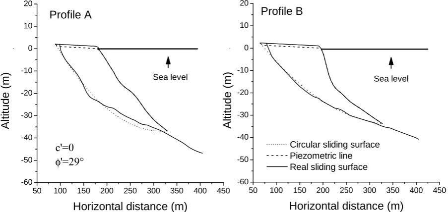
Fig. 6. Deˇgirmendere coastline before the slide (solid line) and footprint of the sliding mass body (dashed line) as reconstructed by Rathje et al. (2004) and by Cetin at al. (2004). Profiles A and B correspond to the vertical-cross sections analysed in the paper.
one solution for the problem, which can be rephrased by stat-ing that they restrict their searchstat-ing space to only one point, which is a not advisable practice to find a point of minimum.
5 Applications to idealized cases
The cases taken into account for the application of our method are initially the same as those that were analysed in TM2006, since this enables us to make proper comparisons. A slope of about 30◦with an arc-like sliding surface is rep-resented in Fig. 2. The body is homogeneous and may be partially submerged under a layer of water with a possible piezometric level that is depicted by a dashed piecewise line. This profile is studied for three different situations: case 1 corresponds to a dry body with null pore pressure and with no external forces applied; case 2 is the case of a body un-der the load of a thin water layer applied on the toe side; in case 3 a seismic load is considered (k=0.368,ψ=42.8◦). The stability is studied by means of the classical method by Spencer and by means of the TM method (Tinti and Manucci, 2006), and, in addition, by using the five more different ap-proaches illustrated in the previous section, i.e. by inverting the “block” system. The discretization of the computational domainxbeg, xend
Table 3. Stability results for the Deˇgirmendere slide body in the pre-earthquake conditions. Profiles A and B are shown in Figs. 6 and 7. All methods give equivalent results: the body is extremely stable on both profiles. Cells with bold characters contain the MLD values.
Method Profile A Profile B
F 1 F δ
Spencer 5.963 0.0680 7.127 0.0525 T&M 5.966 0.0672 7.115 0.0523 T&M-new 5.961 0.0672 7.127 0.0523 T&M-Xsin 5.961 0.0672 7.127 0.0523 T&M-Xcos 5.961 0.0672 7.127 0.0523 T&M-Ecos 5.956 0.0976 7.125 0.1938 T&M-Acos 5.939 0.3049 7.126 0.7750
All results are summarized in Table 1 where the values of the minimum lithostatic deviations and of the corresponding safety factors are given. Technically, the complete solution includes the further specification of the computed unknown functionsE(x), X(x), A(x)and P (x). For case 1, these curves are provided in Fig. 3. The body results to be sta-ble in case 1 and even more stasta-ble in case 2, where the water load stabilizes the slope, while it is unstable in case 3 due to the seismic load.
As it may be seen from Table 1, the classical Spencer’s method gives results quite different from all our approaches, both in terms of MLD (remarkably higher) and in terms ofF (higher). Judged through the MLD principle, this method re-sults to be the worst. On the other hand, the rere-sults of all our methods are quite close to one another. As already remarked, the methods T&M and T&M-new compute the solution ex-actly to the same problem, but via different numerical algo-rithms. Hence, the differences in the corresponding results are only due to numerical rounding errors. It is further in-teresting to note that the methods T&M-new and T&M-Xsin assume the same three-term expansion forX(x), though us-ing different choices for known and unknown coefficients. The results are almost identical, which is explained by the fact that these methods explore the same searching space to find the MLD, though by means of a different searching grid. Further, the worst results for our methods are the ones de-riving from the weighted cosine expansions of the function EandA(T&M-Ecos, T&M-Acos). Finally, we observe that the minimum values ofδare obtained by the method T&M-Xcos for all three cases, which is suggestive that the weighted cosine expansion ofXis the best possible assumption among the ones examined here.
Looking at the graphs of Fig. 3, it is clear that the three si-nusoidal expansion methods (T&M, T&M-new, T&M-Xsin) are almost equivalent. The weighted cosine expansion for the forceX, which is our best solution, departs slightly from the others in the up-hill part of the slide regards the force
Table 4. Stability results for the Deˇgirmendere slide body under conditions presumably acting during the earthquake (k=0.45, ψ =-22◦) and the consequent tsunami produced by the earthquake itself (sea level lowers by 1 m). All methods, including the traditional Spencer’s method, produce similar values for the factor of safety, and the conclusion is that both profiles are unstable. Cells with bold characters contain the MLD values.
Method Profile A Profile B
F δ F δ
Spencer 0.908 0.1728 0.989 0.1714 T&M 0.906 0.1621 0.989 0.1630 T&M-new 0.906 0.1623 0.988 0.1625 T&M-Xsin 0.906 0.1623 0.988 0.1625 T&M-Xcos 0.906 0.1623 0.988 0.1626 T&M-Ecos 0.906 0.1631 0.988 0.1696 T&M-Acos 0.904 0.1861 0.987 0.2592
and torque functions, but it is quite similar as far as the bot-tom pressureP is concerned. Worth of notice is that for all the cosine methods (T&M-Xcos, T&M-Ecos, T&M-Acos) there is an irregularity of the curves in correspondence with the thinning of the sliding mass at the horizontal distance of about 75 m (see Fig. 2). This is due to the fact that, in this expansion, cosines are corrected by a normalised weight (proportional to the slide thickness), that changes abruptly around that value of the abscissa. We remark further that the last two methods (T&M-Ecos, T&M-Acos) give curves very different from all the others, with the largest discrepancies observable for the torque profiles.
5.1 Stratification
The stratification of the soil is incorporated in the formula-tion of the limit-equilibrium problem presented here through the coefficientsα(x)andβ(x)of the formulas (9) and hence entered in the final discrete system of Eqs. (19), (23) and (24) through the matrices AE, AX, and AAand the vectors bE, bX,
and bA. Therefore, system (19), (23) and (24) is perfectly
5 0 1 0 0 1 5 0 2 0 0 2 5 0 3 0 0 3 5 0 4 0 0 4 5 0 - 6 0
- 5 0 - 4 0 - 3 0 - 2 0 - 1 0
0
1 0 2 0
S e a l e v e l S e a l e v e l
A
lt
it
u
d
e
(
m
)
H o r i z o n t a l d i s t a n c e ( m )
C i r c u l a r s l i d i n g s u r f a c e P i e z o m e t r i c l i n e R e a l s l i d i n g s u r f a c e
5 0 1 0 0 1 5 0 2 0 0 2 5 0 3 0 0 3 5 0 4 0 0 4 5 0
- 6 0 - 5 0 - 4 0 - 3 0 - 2 0 - 1 0
0
1 0 2 0
P r o f i l e A
A
lt
it
u
d
e
(
m
)
H o r i z o n t a l d i s t a n c e ( m )
P r o f i l e B
c'=0
φ
'=29°
Fig. 7. Vertical cross sections of the profiles A and B of Fig. 6. The soil parameter c’,φ’,ρ are constant over the sliding mass, with
respective values of 0 kPa, –22◦and 20 kNm−3. The sliding surfaces are assumed to be circular (dashed line) and the sliding bodies are partly submerged.
of stabilisation for the body. All results are given in Table 2. Very interestingly we confirm here that Spencer’s method de-parts from all the others, that all the sine expansion cases give similar results, and that the best results are obtained through the weighted cosine expansion of the vertical inter-slice force X(T&M-Xcos).
5.2 A real case
In this section we apply the block-matrix method to a real case, that is the case of a slide that was released in Deˇgirmendere, a coastal village in the Izmit Gulf, Turkey, as the result of a disastrous M=7.4 earthquake, that af-fected the north-western part of Turkey on 17 August 1999. Deˇgirmendere is located in the south coast of the Izmit Gulf between the Karam¨ursel Basin and the Eastern Basin (see Fig. 5). The slide involved a segment of coast about 300 m long and 75 m wide, and carried into the sea a multi-storey hotel and two adjacent buildings. It produced a local tsunami. In Fig. 6 the coastline before and after the slide is sketched, together with two profiles A and B intersecting the coast, along which we take the vertical cross-sections depicted in Fig. 7 (Tinti et al., 2006). The earthquake produced a tsunami that was observed in the entire Izmit bay. The tsunami was not catastrophic, with measured run-up heights comprised in the range of 1–3 m. The stability analysis that was con-ducted by Tinti et al. (2006) showed that the earthquake shak-ing, with peak ground acceleration estimated to be about 0.45 g, was the cause of the slide, and in turn of the asso-ciated tsunami that added its effect locally (run-up heights larger than 10 m) to the one produced by the earthquake (see
also Wrigth and Rathje, 2003). It was further speculated that the lowering of the sea level associated with the earthquake tsunami could have acted as an additional factor of destabili-sation for the slide.
The two cross-sections A and B have been analysed with the new computational approach described before and the re-sults are synthesised in Tables 3 and 4. Two cases are con-sidered for both profiles: first, the stability of the slope is evaluated in the pre-earthquake condition with no seismic shaking and no effect of the seismic-origin tsunami (Table 3); secondly, the stability is analysed under the condition of an active seismic load (k=0.45, ψ =–22◦) and of an ongoing tsunami causing a destabilising sea level decrease of 1 m (Ta-ble 4). The material properties of the body were measured by Cetin et al. (2004) during a post-earthquake survey. Compar-ing the results of all methods, one sees that the methods pro-viding the highest values of the lithostatic deviation are con-firmed to be Spencer, T&M-Ecos and T&M-Acos. However, one also finds that the computed values of the factor of safety are quite similar, though the values of theδdepart somewhat from one another. This means that for this particular appli-cation using one method or another is nearly equivalent for practical purposes.
6 Conclusions
MLD principle provides a criterion to find the best solution and the corresponding safety factor for the slope under study. In this paper we have worked within the frame of the MLD approach and on discretising the basic system of equilibrium equations. We have obtained a linear set of algebraic equa-tions in the block matrix form (19), (23) and (24) that is quite easy to solve by the standard real-matrix inversion codes. One of the most relevant result of our analysis is the expres-sion of the problem through the formulation (19), (23) and (24). It has a number of great advantages: 1) it may be ap-plied to a wide range of slopes and of conditions, since it accounts for dry and wet soils, for external distributed loads such as those exerted by a water layer or by seismic shak-ing; 2) it handles bodies with arbitrary geometry, which in-cludes arbitrary bottom profiles; 3) it accounts also for an arbitrary body stratification (which means that, since layers can be separated by arbitrary interfaces and be made as thin as we wish, it can also be adapted to treat a totally heteroge-neous body with variables depending on the horizontal and vertical coordinatesx andz); 4) the formulation is flexible enough to allow one to make a wide range of assumptions on the unknown vectors by expanding one of these (eitherX, or E, orA) over a set ofmbase-functions, and consequently to explore the corresponding (m-1)D searching space. For illustrative reasons we restricted all our applications tom=3 expansions which lead to 2-D searching space of the type IF×Iq.
Comparison of our results with traditional methods is lim-ited to the Spencer’s method that was seen to be one of the best classical approaches (TM2006). This comparison shows that Spencer’s method provides always larger values of litho-static deviation and hence, if the MLD principle is adopted, worse determinations of the safety factor. For all cases ex-amined in this paper, expansions of the unknownsEandA seem to miss the MLD and then are probably not advisable. When we considered the homogeneous body already studied in TM2006, we found that the most convenient assumption is the one we called T&M-Xcos, and the same conclusion was also reached for the ideal stratified bodies (heterogeneous as regards either density, or cohesion, or friction angle). When we considered the real case of the Deˇgirmendere slide that was caused by a tsunamigenic earthquake and itself caused a local tsunami, we found that one can confirm the same rank-ing of the methods in terms of MLD, but, in spite of this, all methods, inclusive Spencer’s, lead to very similar values of the safety factor. The fact thatF is rather insensitive toδ, can be also stated in the inverse way that very small variations of Fproduce very large changes ofδ. Whether this is due to the geometrical or physical properties of the body or is the appar-ent effect of the limitedness of the searching space spanned in this application is a question that can be answered by mak-ing further assumptions on the unknowns, e.g. by increasmak-ing the numbermof the coefficients in the proposed expansions, which is a subject of further research.
Acknowledgements. This research has been financed on funds from the European project TRANSFER n.037058 and the project FIRB RBAP04EF3A 004 of the Italian Ministry of University and Research (MIUR).
Edited by: K.-T. Chang
Reviewed by: A. Volkwein and another anonymous referee
References
Bishop, A. W.: The use of the slip circle in the stability analysis of slopes, Geotechnique, 5, 7-17,1955
Cetin, K. O., Isik, N., Unutmaz, B.: Seismically induced land-slide at Deirmendere Nose, Izmit bay during Kocaeli ( ´ Yzmit)-Turkey earthquake, Soil Dynamics and Earthquake Engineering, 24, 189–197, 2004.
Chen, Z. and Morgenstern, N. R.: Extension to the generalized method of slices for stability analysis, Can. Geotech. J., 20, 104– 119,1983.
Chen, Z., Mi, H., and Wang, X.: A three-dimensional limit equilibrium method for slope stability analysis, Chinese J. Geotech.Engrg., 23, 525–529, 2001.
Duncan, J. M. and Wright, S. G.: The accuracy of equilibrium meth-ods of slope stability analysis, Engrg. Geol., 16, 5–17, 1980. Fellenius, W.: Erdstatische Berechnungen mit Reibung und
Koha-sion, Ernst, Berlin (in German), 1927.
Graham, J.: Methods of stability analysis, In “Slope instability”, edited by D. Brunsden and D.B. Prior, Wiley-Intersciences Pub-lication, Wiley & Sons, Chichester, 171–215, 1984.
Janbu, N.: Slope stability computations, Soil Mech. And Found. Engrg. Rep., The Technical University of Norway, Trondheim, Norway, 1968.
Jiang, J. C. and Yamagami, T.: Three-dimensional slope stability analysis using an extended Spencer method, Soils and Founda-tions, 44, 127–135, 2004.
Karaulov, A. M.: Statement and solution of the stability problem for slopes and embankments as a linear-programming problem, Soil Mechanics and Foundation Engineering, 42, 75–80, 2005. Leshchinsky, D. and Huang, C.: Generalized three dimensional
slope stability analysis, J. Geotech. Engrg., ASCE, 118, 1748– 1764, 1992.
Morgenstern, N. R. and Price, V. E.: The analysis of the stability of general slip surfaces, Geotechnique, 15, 79–93, 1965.
Pink, M. N.: Analysis of slope stability by the method of limit-ing equilibrium, Soil Mechanics and Foundation Engineerlimit-ing, 44, 99–104, 2007.
Rathje, E. M., Karatas, I., Wright, S. G., and Bachhuber, J.: Coastal Failures during the 1999 Kocaeli Earthquake in Turkey, Soil Dyn. Earthqu. Eng., 24(9–10), 699–712, 2004.
Spencer, E.: A method of analysis of the stability of embankments assuming parallel interslice forces, Geotechnique, 17, 11–26, 1967.
Tinti, S. and Manucci, A.: Gravitational stability computed through the limit equilibrium method revisited, Geophysical International Journal, 164, 1–14 , 2006.
(tectonic) and local (mass instabilities) causes, Marine Geology, 225, 311–330, 2006.
Wright, S. G. and Rathje, E. M.: Triggering mechanisms of slope instability and their relationship to earthquakes and tsunamis, Pure and Applied Geophysics, 160, 1865–1877, 2003.
Zheng, H., Liu, D. F., and Li, C. G.: On the assessment of failure in slope stability analysis by finite element method, Technical note, Rock Mechanics and Rock Engineering, doi:10.1007/s00603-007-0129-8, 2007.