On some reduced order models for packed separation processes

(1)

UCL

i ~ ~l

d z : ]

UNIVERSITY COLLEGE LONDON

DEPARTMENT OF CHEMICAL & BIOCHEMICAL ENGINEERING

O

n

S

o m e

R

e d u c e d

O

r d e r

M

o d e l s f o r

P

a c k e d

S

e p a r a t io n

P

r o c e s s e s

by Leonardo de Gil Torres, MSc

A thesis submitted for the degree of

Doctor of Philosophy

in the

University of London

Department of Chemical & Biochemical Engineering University College London

(2)

ProQuest Number: 10106825

INFORMATION TO ALL USERS

The quality of this reproduction is dependent upon the quality of the copy submitted.

In the unlikely event that the author did not send a complete manuscript and there are missing pages, these will be noted. Also, if material had to be removed,

a note will indicate the deletion.

uest.

ProQuest 10106825

Published by ProQuest LLC(2016). Copyright of the Dissertation is held by the Author.

This work is protected against unauthorized copying under Title 17, United States Code. Microform Edition © ProQuest LLC.

ProQuest LLC

789 East Eisenhower Parkway P.O. Box 1346

(3)

Abstract 2

ABSTRACT

The use of packed-bed separation columns as a liquid-gas contact system in

absorption and distillation has steadily increased in the chemical and process

industries and with it the need for tools for their adequate design and control.

The mathematical models for packed separation columns are known for their

large dimensionality. This can pose a problem when one considers the design

and/or optimisation of systems involving more than one column or a single

large column. The use of reduced-order models came as an answer to this

problem. Reduced-order models presented to date do not rigorously solve the

mass transfer subproblem.

Four generalised steady-state reduced-order models for separation processes

in packed columns are developed and compared in this work. The models are

based on the two film theory of mass transfer and the more rigorous of them

have as a starting point one of the so called rate based methods. The mass

and energy transfer rates across the vapour liquid interface are evaluated by

means of different approximate solutions of the Maxwell-Stefan equations for

steady-state, unidirectional mass transfer. The differential equations of the

models are converted into algebraic equations through the application of the

orthogonal collocation procedure on the spatial variable. The resulting system

of algebraic equations is subsequently solved using a modification of the

Powell hybrid method. Three case studies dealing with distillation columns are

presented but the models are easily modified to work with other separation

processes (e.g., absorption).

The results of the simulations indicated a clear advantage when using more

rigorous methods for the computation of the interphase mass transfer rates.

Their inclusion in the reduced-order models improved the convergence

characteristics of the solution with respect to the number of collocation points

and also increased the robustness of the models in converging towards the

solution. These improvements were obtained without increasing significantly

the time spent in the simulations when compared with a model using an

(4)

Gabriel

Q a b i i i e û

^ e t o Quedes e ^ o n a M o %as(:os

é 20 de m a x

£ de deeejax que a % do H0220 amox

L M atéxia pxima desta cançào

^ iq u e a bxi^hax

£ é pxâ voce

£ pxâ todo mundo que quex txa^ex assim

lA pag no coxaçâo

uU eu poqueno amofi

£ de voce me hmbxax

ÇToda veg que a vida mandax ofto/i pm ecu

£ s tx ê la da manlia

u Ü eu pequeno gxande amox

Q u e c voce Qabxieê

% d pode/t sex fiivxe como a gente quig

Quexo te vex M ia

(5)

Acknowledgements

ACKNOWLEDGEMENTS

I would like to express my sincere gratitude to all those who provided support

throughout this work at University College London. Special thanks go to my

supervisor, Dr. David Bogle, for his constructive criticism during my research

and in the preparation of this thesis and, above all, for his friendship.

I would also like to thank the Universidade Federal Rural do Rio de Janeiro,

Brazil, which gave me the opportunity to come to England to develop this

research.

I am very grateful to all the members of the ‘United Nations of Room 305’ for

making my time at UCL so enjoyable. A special thought goes to Sam & Jackie,

Kenny & Bega, Firoozeh, Robert, Sabine, Annette & Chris, Rafael & Paty,

Patrick, Carlos and Pat Bloomfield.

A word of gratitude to my parents and my family in Brazil for their love. It is

extended to my family in London, Fernando, Norma (Livia) & Juliana, and to my

‘Brazilian’ friends Firton, Rafael & Andréa, Ney & Maria, Rodrigo & Valeria,

Angela & Carolina, Carlos & Margarita, etc.. They did not allow the banzo to

take over.

I am forever indebted to Cynésia for her endless patience, support and love.

I finally acknowledge the Coordenaçâo de Aperfeiçoamento de Pessoal de

Nivel Superior - CAPES - BRAZIL (the Federal Agency for Post-graduate

(6)

Acknowledgements

(7)

Table of Contents

INDEX OF FIGURES

Figure 2.1 Sketch of the equilibrium stage 25

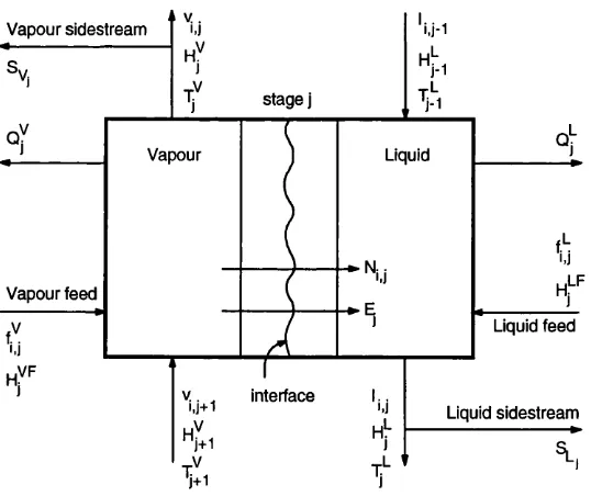
Figure 2.2 Sketch of the nonequilibrium stage 38

Figure 2.3 Composition and temperature profiles in the region of the

interface 40

Figure 2.4 Method decision diagram [Haas (1992)] 47

Figure 3.1 Definition of some variables on a tray 53

Figure 3.2 Two-film model of a packed column 62

Figure 3.3 Rectification section of a distillation column with a total

condenser 63

Figure 4.1 Interaction effects on diffusion in multycomponent systems

[adapted from Taylor and Krishna (1993)] 74

Figure 4.2 Mole fractions close to the interface during mass transfer 78

Figure 4.3 Interface region according to the film theory (film of

thickness 4 79

Figure 4.4 Mass and energy transfer across a phase boundary 102

Figure 5.1 Geometric properties of typical structured packings, (a) Flow

channel cross section, (b) Flow channel arrangement

[adapted from Fair and Bravo (1990)] 124

Figure 6.1 Sketch of the distillation column 126

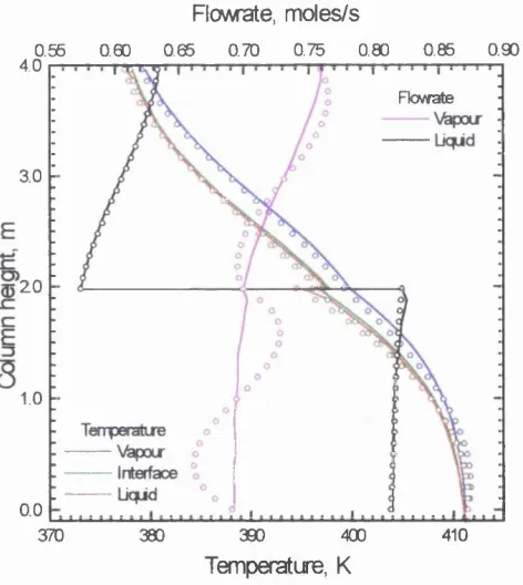
Figure 9.1 Comparison between the initial profiles (o o o) and the profiles obtained using R0M1 with n=m=^0 (--- ) for example 1. Liquid mole fraction profiles 158

Figure 9.2 Comparison between the initial profiles (o o o) and the profiles obtained using R0M1 with n=m=10 (--- ) for

example 1. Temperature and flowrate profiles 158

Figure 9.3 Comparison between the initial profiles (o o o) and the profiles obtained using R0M1 with n=m=^0 (--- ) for example 1. Interphase mass transfer rate profiles 159

Figure 9.4 Comparison between the initial profiles (o o o) and the profiles obtained using R0M2 with n=m=10 (--- ) for

example 1. Liquid mole fraction profiles 159

Figure 9.5 Comparison between the initial profiles (o o o) and the profiles obtained using R0M2 with n=m=^0 (--- ) for example 1. Temperature and flowrate profiles 160

(14)

Index of Figures_________________________________________________________13 Figure 9.7 Comparison between the initial profiles (o o o) and the

profiles obtained using ROMS with n=m=10 ( ) for

Figure 9.8 Comparison between the initial profiles (o o o) and the profiles obtained using ROMS with n=m=10 (--- ) for

Figure 9.9 Comparison between the initial profiles (o o o) and the profiles obtained using ROMS with n=m=^0 (--- ) for example 1. Interphase mass transfer rate profiles 162

Figure 9.10 Comparison between the initial profiles (o o o) and the profiles obtained using R0M4 with n=m=^0 (--- ) for example 1. Liquid mole fraction profiles 162

Figure 9.11 Comparison between the initial profiles (o o o) and the profiles obtained using R0M4 with n=m=10 (--- ) for example 1. Temperature and flowrate profiles 16S

Figure 9.12 Comparison between the initial profiles o o) and the profiles obtained using R0M4 with n=m=^0 (--- ) for example 1. Interphase mass transfer rate profiles 16S

Figure 9.IS R0M1 - Comparison between the solution obtained with

n=m=2 ( o o o ) and the solution obtained using n=m=10 (---) for example 1. Liquid mole fraction profiles 165

Figure 9.14 R0M1 - Comparison between the solution obtained with

n=m=2 ( o o o ) and the solution obtained using n=m=^0 (---)

for example 1. Temperature profiles 165

n=m=2 ( o o o ) and the solution obtained using n=m=^0 (---) for example 1. Interphase mass transfer rate profiles 166

n=m=2 ( o o o ) and the solution obtained using n=m=10 (---) for example 1. Liquid mole fraction profiles 166

n=m=2 ( o o o ) and the solution obtained using n=m=10 (--- ) for example 1. Temperature and flowrate profiles 167

n=m=2 ( o o o ) and the solution obtained using n=m=^0 (---) for example 1. Interphase mass transfer rate profiles 167

(15)

Index of Figures_________________________________________________________14 Figure 9.20 R0M4 - Comparison between the solution obtained with

n=m=2 ( o o o ) and the solution obtained using n=m=^0 (--- ) for example 1. Temperature and flowrate profiles 168

n=m=2 ( o o o ) and the solution obtained using n=m=^0 (--- ) for example 1. Interphase mass transfer rate profiles 169

Figure 9.22 Comparison between the solution for example 1 obtained

with model R0M1 (o o o) and the solution obtained with model R0M4-- (--). Liquid mole fraction profiles (n=m=10) 170

with model R0M1 (ooo)and the solution obtained with model R0M4 (---). Temperature and flowrate profiles (n=m=10) 170

with model R0M1 (o o o) and the solution obtained with model R0M4 (---). Interphase mass transfer rate profiles

{n=m=^0) 171

Figure 9.25 Comparison between the solution for example 1 obtained with model R0M2 (o o o) and the solution obtained with model R0M4 (--). Liquid mole fraction profiles {n=m=^0) 171 Figure 9.26 Comparison between the solution for example 1 obtained

with model R0M2 (ooo) and the solution obtained with model R0M4 (---). Temperature and flowrate profiles (n=m=10) 172

Figure 9.27 Comparison between the solution for example 1 obtained with model R0M2 (o o o) and the solution obtained with model R0M4 (---). Interphase mass transfer rate profiles

(n=m=10) 172

with model ROMS (o o o) and the solution obtained with model R0M4 (--). Liquid mole fraction profiles (n=m=^0). 173 Figure 9.29 Comparison between the solution for example 1 obtained

with model ROMS (ooo) and the solution obtained with model R0M4 (---). Temperature and flowrate profiles (n=m=^0) 173 Figure 9.30 Comparison between the solution for example 1 obtained

with model ROMS (o o o) and the solution obtained with model R0M4 (---). Interphase mass transfer rate profiles

(A7=A77=10) 174

Figure 9.31 Evolution of the Euclidean norm of the vector of functions with the iteration number. Solutions of example 1 with ten

(16)

Index of Figures 15 Figure 9.32 Evolution of the Euclidean norm of the vector of functions

with the iteration number. Solutions of example 1 with six

internal collocation points per section 175

Figure 9.33 Evolution of the Euclidean norm of the vector of functions

with the iteration number. Solutions of example 1 with four

with the iteration number. Solutions of example 1 with three

with the iteration number. Solutions of example 1 with two

Figure 10.1 Comparison between the initial profiles (o o o) and the profiles obtained using R0M1 with n=m=^0 (--- ) for

Figure 10.2 Comparison between the initial profiles (o o o) and the profiles obtained using R0M1 with n=m=10 (--- ) for example 2. Temperature and flowrate profiles 180

Figure 10.3 Comparison between the initial profiles (o o o) and the profiles obtained using R0M1 with n=m=^0 (--- ) for example 2. Interphase mass transfer rate profiles 181

Figure 10.4 Comparison between the initial profiles (o o o) and the profiles obtained using R0M2 with n=m=^0 (--- ) for example 2. Liquid mole fraction profiles 181

Figure 10.5 Comparison between the initial profiles (o o o) and the profiles obtained using R0M2 with n=m=^0 (--- ) for example 2. Temperature and flowrate profiles 182

Figure 10.6 Comparison between the initial profiles (o o o) and the profiles obtained using R0M2 with n=m=^0 (--- ) for example 2. Interphase mass transfer rate profiles 182

Figure 10.7 Comparison between the initial profiles (o o o) and the profiles obtained using R0M3 with n=m=^0 (--- ) for

Figure 10.8 Comparison between the initial profiles (o o o) and the profiles obtained using R0M3 with n=m=^0--- (--- ) for example 2. Temperature and flowrate profiles 183

(17)

Index of Figures_________________________________________________________16 FigurelO.10 Comparison between the initial profiles (o o o) and the

profiles obtained using R0M4 with n=m=^0 (--- ) for

Figure10.11 Comparison between the initial profiles (o o o) and the profiles obtained using R0M4 with n=m=^0 (--- ) for example 2. Temperature and flowrate profiles 185

Figure10.12 Comparison between the initial profiles (o o o) and the profiles obtained using R0M4 with n=m=^0 (--- ) for example 2. Interphase mass transfer rate profiles 185

FigurelO.13 R0M1 - Comparison between the solution obtained with

n=m=3 ( o o o ) and the solution obtained using n=m=10 (--- ) for example 2. Liquid mole fraction profiles 187

Figure10.14 R0M1 - Comparison between the solution obtained with

n=m=3 ( o o o ) and the solution obtained using n=m=10 (--- )

FigurelO.16 R0M2 - Comparison between the solution obtained with

n=m=3 ( o o o ) and the solution obtained using n=m=^0 (--- ) for example 2. Temperature and flowrate profiles 189

n=m=3 ( o o o ) and the solution obtained using n=m=10 (--- ) for example 2. Interphase mass transfer rate profiles 189

n=m=3 ( o o o ) and the solution obtained using n=m=10 (--- ) for example 2. Temperature and flowrate profiles 190

Figure10.22 Comparison between the solution for example 2 obtained

(18)

Index of Figures 17 Figure10.23 Comparison between the solution for example 2 obtained

with model R0M1 (o o o) and the solution obtained with model R0M4 (---- ). Temperature profiles {n=m=^0) 192 Figure10.24 Comparison between the solution for example 2 obtained

with model R0M1 (o o o) and the solution obtained with model R0M4 (---). Interphase mass transfer rate profiles

(A7=n7=10) 193

with model R0M2 (o o o) and the solution obtained with model R0M4 (---- ). Liquid mole fraction profiles (n=/7?=10) 193

with model R0M2 (ooo) and the solution obtained with model

R0M4 (---). Temperature and flowrate profiles {n=m=^0) 194 Figure10.27 Comparison between the solution for example 2 obtained

with model R0M2 (o o o) and the solution obtained with model R0M4 (---). Interphase mass transfer rate profiles

{n=m=^0) 194

Figure10.28 Comparison between the solution for example 2 obtained with model R0M3 (o o o) and the solution obtained with model R0M4 (---- ). Liquid mole fraction profiles (n=m=^0). 195 Figure10.29 Comparison between the solution for example 2 obtained

with model R0M3 (ooo) and the solution obtained with model

R0M4 (--- ). Temperature and flowrate profiles (n=m=10) 195

(n=A77=10) 196

Figure10.31 Evolution of the Euclidean norm of the vector of functions

with the iteration number. Solutions of example 2 with ten

(19)

Index of Figures_________________________________________________________1^

Figure 11.1 Comparison between the initial profiles (o o o) and the profiles obtained using R0M1 with n=m=^0 ( ) for

Figure 11.2 Comparison between the initial profiles o o) and the profiles obtained using R0M1 with n=nn=^0 ( ) for example 3. Temperature and flowrate profiles 202

Figure 11.3 Comparison between the initial profiles o o) and the profiles obtained using R0M1 with n=m=^0 ( ) for example 3. Interphase mass transfer rate profiles 203

Figure 11.4 Comparison between the initial profiles (o o o) and the profiles obtained using R0M2 with n=m=6 (--- ) for example

3. Liquid mole fraction profiles 203

Figure 11.5 Comparison between the initial profiles (o o o) and the profiles obtained using R0M2 with n=m=6 (--- ) for example

3. Temperature and flowrate profiles 204

Figure 11.6 Comparison between the initial profiles (o o o) and the profiles obtained using R0M2 with n=m=6 (--- ) for example

3. Interphase mass transfer rate profiles 204

Figure 11.7 Comparison between the initial profiles (o o o) and the profiles obtained using R0M3 with n=m=^0 ( ) for

Figure 11.8 Comparison between the initial profiles (o o o) and the profiles obtained using R0M3 with n=m=^0 (---) for example 3. Temperature and flowrate profiles 205 Figure 11.9 Comparison between the initial profiles (o o o) and the

profiles obtained using R0M3 with n=m=10 (---) for

example 3. Interphase mass transfer rate profiles 206

Figurel 1.10 Comparison between the initial profiles (o o o) and the profiles obtained using R0M4 with n=m=^0 (---) for

Figurel 1.11 Comparison between the initial profiles {o o o) and the profiles obtained using R0M4 with n=m=10 (---) for

Figurel 1.12 Comparison between the initial profiles (o o o) and the profiles obtained using R0M4 with n=m=10 (---) for

(20)

Index of Figures_________________________________________________________1^

Figurel 1.13 R0M1 - Comparison between the solution obtained with

n=m=3 (o o o ) and the solution obtained using n=m=^0 (--- ) for example 3. Liquid mole fraction profiles 209

n=m=3 (o o o ) and the solution obtained using n=m=^0 (--- )

n=m=3 (o o o ) and the solution obtained using n=m=10 (--- ) for example 3. Interphase mass transfer rate profiles 210

n=m=3 (o o o) and the solution obtained using n=m=6 (--- ) for example 3. Liquid mole fraction profiles 210

n=m=3 (o o o) and the solution obtained using n=m=6 (--- ) for example 3. Temperature and flowrate profiles 211

n=m=3 (o o o) and the solution obtained using n=m=6 (--- ) for example 3. Interphase mass transfer rate profiles 211

n=m=3 ( o o o ) and the solution obtained using n=m=^0 (--- ) for example 3. Liquid mole fraction profiles 212 Figurel 1.20 R0M4 - Comparison between the solution obtained with

n=m=3 (o o o ) and the solution obtained using n=m=10 (--- ) for example 3. Temperature and flowrate profiles 212

n=m=3 ( o o o ) and the solution obtained using n=m=10 (--- ) for example 3. Interphase mass transfer rate profiles 213

Figurel 1.22 Comparison between the solution for example 3 obtained

with model R0M1 (o o o) and the solution obtained with model R0M4--(---- ). Liquid mole fraction profiles {n=m=6) 214 Figurel 1.23 Comparison between the solution for example 3 obtained

with model R0M1 (o o o) and the solution obtained with model R0M4--(---- ). Temperature profiles (n=m=6) 215 Figurel 1.24 Comparison between the solution for example 3 obtained

with model R0M1 (ooo)and the solution obtained with model R0M4 (---). Interphase mass transfer rate profiles (n=m=6) 215 Figurel 1.25 Comparison between the solution for example 3 obtained

(21)

Index of Figures 20 Figurel 1.26 Comparison between the solution for example 3 obtained

with model R0M2 (o o o) and the solution obtained with model R0M4 (--- ). Temperature and flowrate profiles

(/7=/7?=6) 216

{n=m=6) 217

with model R0M3 (o o o) and the solution obtained with model R0M4 (---). Liquid mole fraction profiles (n=m=6). 217 Figurel 1.29 Comparison between the solution for example 3 obtained

with model R0M3 (o o o) and the solution obtained with model R0M4 (---). Temperature and flowrate profiles

(n=/77=6) 218

{n=m=Q) 218

Figurel 1.31 Evolution of the Euclidean norm of the vector of functions

with the iteration number. Solutions of example 3 with ten

(22)

Index of Tables 21

INDEX OF TABLES

Table 4.1 Determinacy coefficients [adapted from Smith and Taylor

(1983)] 82

Table 5.1 Coefficients Cn for the series in equation (5.41) 115 Table 5.2 Atomic diffusion volumes [Reid etal. (1987)] 119 Table 5.3 Critical surface tension of packing materials [Perry et al.

(1984)] 123

Table 9.1 Specifications for case study 1 156

Table 9.2 Example 1 - Summary of results 164

Table A3.1 CPU time (s) spent in the simulations of case study 1 255

Table A3.2 CPU time (s) spent in the simulations of case study 2 255

(23)

Chapter 1 - Introduction 22

1 - INTRODUCTION

In the beginning, distillation was just a rudimentary technique for the production

of liquors through the concentration of the alcoholic content of beverages.

With the passage of the years, distillation developed tremendously to become

the most used and important unit operation of the chemical and process

industries.

Distillation was performed traditionally in tray columns and only in recent years

an increase in the use of packed distillation columns has been seen. For this

historical reason almost all the design and/or simulation of packed distillation

columns are made using techniques developed for tray columns.

Considering the increasing complexity of chemical processes, together with the

need to incorporate energy integration in the design, there is clearly an

opportunity for the introduction of optimisation procedures. Equation-based

optimisation requires the use of process models that accurately describe the

phenomena taking place in the equipment. However, the optimisation of

systems involving more than one column or a single large column can be

extremely time consuming due to the complexity and large dimensionality of the

mathematical model to be solved. The same concern with the size of the

models exists in control system synthesis studies where repeated simulations

are necessary.

This need for more efficient process models requiring less solution effort gave

rise to the development of several procedures for the reduction of the order of

the models. It is clear that, on one hand, the reduced-order models must retain

certain properties from the rigorous models (e.g., must retain the necessary

gradient information of the rigorous model to ensure convergence to the

optimum of the rigorous model) but, on the other hand, the dimensionality of

(24)

Chapter 1 - Introduction 23 Orthogonal collocation is one of the best known methods for the numerical

solution of differential equations in Chemical Engineering models. In the last

ten years or so, there has been a great interest on the development of reduced-

order models for distillation columns based on the orthogonal collocation

procedure. Apart from a small number of exceptions, this effort has been

concentrated in modeling tray columns.

The aim of this work is to develop steady-state reduced-order models for

packed separation processes in general, and for distillation in particular. These

reduced-order models are intended to incorporate in their core a more rigorous

approach (when compared with the current standards for reduced-order

models) in the evaluation of the interphase mass transfer rates.

As the starting point, in chapter 2, a review of the so called rigorous methods

for multistaged separation columns will be presented. Some emphasis will be

given to the rate based methods as they are intended to be the basis of the

reduced-order models to be developed. This will be followed, in chapter 3, by

an analysis of the reduced-order models based on the orthogonal collocation

method. As already mentioned, most of the work reported in the open literature

deals with tray columns. Nevertheless, there are many lessons to be learned

from these experiences.

The necessary tools to rigorously analyse multicomponent mass transfer are

discussed in chapter 4. These rigorous computations will need to be backed by

the evaluation of several properties of the system. This will be dealt with in

chapter 5.

Chapters 6, 7, and 8 are devoted to a comprehensive description of the

reduced-order models developed in this work while chapters 9, 10, and 11 will

present the results of three case studies.

Finally, in chapter 12, some conclusions on the performance of the reduced-

order models are presented together with some topics that deserve further

(25)

Chapter 2 - Rigorous Methods fo r the Simulation o f Multistaged Separations 24

2- RIGOROUS METHODS FOR THE SIMULATION OF

MULTISTAGED SEPARATIONS

2 .1 - In t r o d u c t io n

One of the basic aims of this work is to develop some models for the simulation

of packed separation processes. As Krishnamurthy and Taylor (1985c) pointed

out, there are basically two different approaches for modelling packed columns.

One of these approaches is to divide the continuous contact device into several

sections, where each of the sections is considered as if it were a stage in a

stagewise contactor. Therefore, as our final aim is to develop some reduced-

order models for the simulation of packed columns, some of the most important

rigorous methods for the simulation of multistaged separation processes will be

presented in this chapter.

In section 2.2 some methods based on the equilibrium-stage concept are

presented while the rate based methods (also known as nonequilibrium stage

models) are presented in section 2.3. Some information on where to find

guidelines on choosing the appropriate method for a specific application is

presented in section 2.4. Finally, in section 2.5, some of the key concepts for

the simulation of packed separation columns are discussed.

2 .2 - Mo d e l s Ba s e d on t h e Eq u il ib r iu m-St a g e Co n c e p t

2.2.1- The equilibrium-stage

Most of the simulation packages available nowadays for the simulation of

multicomponent multistage separations are based on the equilibrium stage

concept.

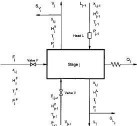
A scheme of a typical equilibrium-stage is presented in Figure 2.1 where the

index j refers to the stage number and / to the component. A separator consists of a number of such stages arranged in a countercurrent cascade. The stages

are numbered down from the top of the column. There is no limitation on the

(26)

Chapter 2 - Rigorous Methods for the Simulation of Multistaged Separations 25 phases leaving the stage are considered to be at thermal and mechanical

equilibrium.

hi

valve V Valve F

— M — ►

— V \A r

Q.

Figure 2.1. Sketch of the equilibrium-stage

2.2.2- Basic equations for the equiiibrium-stage

The equations used to describe the steady state operation of a distillation

column are often referred to as the MESH equations [after the work of Wang

and Henke (1966)]. The MESH acronym stands for:

• Material balance for each component (no equations per stage)

M/,y = ^y-i^/.y-i "I" ^y+iy/,y+i + ^ j ^ i j ~ (^y ^ Lj ) ^ i , j ~ (^y ^ V j ] V i , j (2- "I )

• Equilibrium relation for each component (no equations per stage)

^/,y = ViJ ~ ~ ®

The equilibrium constant, K,y, is usually a complex function of the general form

(27)

Chapter 2 - Rigorous Methods f o r the Simulation o f Multistaged Separations_______ ^

• Mole fraction Summations (one equation per stage)

nc

(^y)y = Z / w -l-O = 0 (2.4)

nc

= 0 (2.5)

• Heat or enthalpy or energy balance (one equation per stage)

H,, . + F jH j - {Lj + S,, )h^ - [v, + S,, )«)' - O, = 0 (2.6)

The enthalpies for each phase are functions of temperature, pressure and

composition and the relations have the general form

(2.7)

H i = H :{T ,.P j,y u ) (2.8)

Equation (2.4) or (2.5) can be replaced by a total material balance obtained

through the combination of equations (2.4), (2.5) and (2.1) summed over the nc

components and over stages 1 to j leading to

(2.9)

/c=1

Sometimes the bubble-point and dew-point equations are used in the solution

method to help in the determination of the stage temperature. These equations

are generated via the combination of the summation equation and the

equilibrium equation, leading to the bubble-point equation

= 0 (2 .10)

/=1

and the dew-point equation

= 0 (2 .11)

(28)

Chapter 2 - Rigorous Methods fo r the Simulation o f Multistaged Separations 27 A countercurrent cascade of Nsequilibrium-stages is represented by Ns(2nc+3) MESH equations. If all F), Zij, T f, P f, and Qj are specified the

system of Ns(2nc+3) nonlinear algebraic equations can be solved for the Ns(2nc+3) variables [%, 7], % and Lj.

2.2.3- Classification of the methods of soiution

There is in the open literature a wide variety of methods to solve the system of

equations presented in the previous section.

Lewis and Matheson (1932) and Thiele and Geddes (1933) are among the first

to address the solution of this system of equations in a stage-by-stage,

equation-by-equation calculation procedure based on equation tearing. These

methods were widely used for hand calculations of simple fractionators with

one feed and two products. In the first attempts to program the Thiele-Geddes

method in a digital computer the solution procedure was often numerically

unstable [Henley and Seader (1981)].

Several improvements in these early methods were presented in the literature

and in a classic study, Friday and Smith (1964) analysed a number of tearing

techniques for the solution of the MESH equations. They concluded that no

single technique is able to handle all types of problems. They also divided the

rigorous methods of solution into four basic classes, namely:

• bubble-point methods (BP);

• sum-rates methods (SR);

• the 2N Newton methods;

• the global Newton or simultaneous correction methods (SC).

The continuous development of new techniques led Haas (1992) to add some

classes to the previous ones, for example:

• inside-out methods;

• relaxation methods;

(29)

Chapter 2 - Rigorous Methods fo r the Simulation o f Multistaged Separations 28 In the following sections a brief description of some of the most important

methods of each class will be presented.

2.2.4- Tridiagonal matrix aigorithm

The tridiagonal matrix algorithm, introduced by Wang and Henke (1966) for

calculating the component and total flowrates, is used in most of the methods

presented in this chapter.

The tridiagonal matrix results from a modification of equation (2.1). The vapour

mole fractions are eliminated from equation (2.1) using equation (2.2) and the

total liquid flowrates are eliminated via substitution of equation (2.9) into

equation (2.1). The resulting equation for component / in stage y is:

where

'o , = - s . .-S v,)-V , (2.13)

k=^

2 < j < N s

M

= - '^y+1 ^ 4 +

{K

+ ®i'/ )^U

k=)

(2.14)

^ < j < N s

(2.15)

^ < j < N s - ^

(2.16)

^ < j < N s

and, for a typical distillation column, x, q = 0, = 0, = 0 and = 0.

Grouping equations (2.12) by component they can be partitioned in nc

(30)

Chapter 2 - Rigorous Methods fo r the Simulation of Multistaged Separations 29

0 0 0 0 ' ' ■ u,,

-'D , 0 • • 0 _^i,2 _Ui.2

0 'D , 0 0 _^/.3 U,3

0 0 'D , _^/.4 U,,4

0

0 _^i.Ns-3 _^i.Ns-3

0 0 0 _^i.Ns-2 _^i.Ns-2

0 0 _^/,A/s-1

0 0 0 0

(2.17)

It is important to emphasise that and ^Dij depend only on the tear variables

(the vector of temperatures and the vector of vapour flow rates) provided that

the values of Kjj are composition independent. If not, compositions from the

previous iteration may be used to estimate the values of K),y.

The output variables of each equation (2.17) are the liquid mole fractions of

component / over the whole column (A/s stages).

There are some solution techniques specially tailored for tridiagonal matrices.

In their work Wang and Henke (1966) recommended the usage of an algorithm

developed by Thomas [Lapidus (1962)]. Boston and Sullivan (1972) presented

a modified Thomas algorithm that is able to handle difficult problems that arise

with columns with a great number of stages and with components whose

absorption factors vary significantly from top to bottom of the column.

2.2.5- Bubble-point methods

In this class of methods the stage temperatures are calculated by solving the

bubble point equation. These methods are generally used for narrow-boiling,

nearly ideal systems.

The Wang and Henke (1966) method uses the tridiagonal matrix to calculate

the compositions and those are used to calculate the temperatures by solving

(31)

Chapter 2 - Rigorous Methods fo r the Simulation o f Multistaged Separations 30 To start the iterative procedure one must assume values for the tear variables.

Frequently the assumption of constant molar interstage flows is a good starting

point. For the initial values of the vector of temperatures it is common practice

to assume a linear variation of the temperature with stage location. The top

temperature can be estimated from the bubble-point of the assumed liquid

distillate product and the bottom temperature from the dew-point of the

assumed bottom product. If the values of Kij are composition dependent one

also needs to estimate the initial liquid and vapour composition profiles.

Alternatively, ideal values of K),y can be used for the first iteration.

The corrected values of the flow rates are computed using equations (2.6) and

(2.9). The procedure is considered to be converged when the variations

between two consecutive sets of temperatures and between two consecutive

sets of flowrates are smaller than a specified tolerance. Frequently successive

substitution is used to update the tear variables.

An interesting alternative is to use the tridiagonal method to calculate the

compositions but a new direct procedure to evaluate temperatures avoiding the

iterative bubble-point temperature determination. This procedure, named the

K^-method, is an approximation of the dew or bubble-point equations and it is

one of the key features of the theta-method of Holland and co-workers [Holland

(1975)]. In the theta-method a convergence promoter, 0, is used to correct the

calculated values of the component flow rates obtained from the solution of the

tridiagonal matrix before they are used in the estimation of the stage

temperatures. The convergence promoter is used to force the overall

component balance as well as the total material balance to be satisfied. This

step is necessary since the flowrates of each component come from different

tridiagonal systems.

2.2.6- Sum-rates methods

The key characteristic of sum-rates' methods is that they use the energy

(32)

Chapter 2 - Rigorous Methods fo r the Simulation o f Multistaged Separations_______ M

to distillation but the reboiler and the condenser must be solved as separate

unit operations [Fonyo et aL (1983)]. Sum-rates’ methods are suited to

modelling absorbers and strippers, being able to simulate some extremely wide

boiling systems containing noncondensables.

Probably the most commonly used sum-rate method is the one developed by

Burningham and Otto (1967). The temperatures are calculated via the solution

of the stage energy balances using a Newton-Raphson technique [a

comprehensive discussion of the Newton-Raphson method and its variants can

be found in Holland (1981)]. Component flow rates are then evaluated using

the tridiagonal matrix algorithm. The component flow rates are then added to

get the total flow rates, a procedure that gives the name of the method (sum-

rates).

2.2.7- 2N Newton methods

Unlike in the bubble-point and sum-rates' methods in the 2N Newton methods

the temperatures and total flow rates are calculated in the same step using a

Newton-Raphson algorithm. The component flow rates are calculated in a

separate step. The name 2N is due to the necessity of writing down two

equations per stage, leading to a total of 2N equations (considering N the

number of stages).

These methods are a good alternative for systems involving the separation of

wide or middle boiling mixtures.

In his formulation Tomich (1970) uses as the first function a combination of the

summation equations for the vapour and liquid compositions [equations (2.4)

and (2.5)]. The second independent function is the stage energy balance. The

total vapour flow rates and the temperatures are chosen as the independent

(33)

Chapter 2 - Rigorous Methods fo r the Simulation o f Multistaged Separations_______ ^

To start the iterative procedure one should guess initial values for the

temperatures and total vapour flow rates. The next step is to evaluate the liquid

compositions using the tridiagonal algorithm. A new set of temperatures and

total vapour flow rates is then obtained via one single iteration of the Newton-

Raphson algorithm. If the norm of the functions is very small and any other

specified criteria are also met the final solution was reached. Otherwise the

whole procedure is repeated on the basis of the new set of temperatures and

total vapour flow rates.

Holland (1981) made a different choice on the functions and variables for the

Newton-Raphson iteration. The independent functions are either the dew-point

or bubble-point equations [equations (2.10) or (2.11)] and the energy balances.

The independent variables are the temperatures and Sy a multiplier defined as

follows:

(2.18)

KJ

CO

The corrected values of the ratio Lj / Vj are used in the absorption and stripping factors employed in the component balances and in the total material balance.

The calculation sequence to be adopted is similar to that of Tomich (1970).

2.2.8- Simultaneous correction methods

The basic characteristic of the simultaneous correction methods is that they

attempt to solve all the MESH equations and variables together. Although they

are the most powerful in solving problems involving nonideal mixtures they

present the weakness of being extremely sensitive to the set of initial values.

Frequently there is the need to use another rigorous method to produce a good

(34)

In the Naphtali-Sandholm method [Naphtali and Sandholm (1971)] the chosen

independent variables for the Newton-Raphson calculation are the stage

temperatures and component liquid and vapour flow rates. The independent

variables are grouped by stage and ordered as presented above. The

independent functions for a stage are the energy balance, one equilibrium

equation for each component and one component balance for each component.

In order to keep the numerical values in the same order of magnitude the

independent functions are written in a normalised form.

These equations are grouped by stage and their order of appearance in the

vector of functions is first the energy balance, second the component balances

and finally the equilibrium equations. This will lead to a total of 2nc+1

equations and variables per stage.

All the variables are solved together producing a Jacobian of size

A / s ( 2 / 7 c + 1 ) x A / s ( 2 / 7 c + 1 ) . Due to the chosen grouping and ordering of the

equations the Jacobian will be sparse with a block-banded structure (blocks of

elements along the main, upper, and lower diagonals).

Starting from an initial set of temperatures and total vapour and liquid flow rates

for each stage the initial component liquid and component vapour flow rates

are calculated using the tridiagonal matrix algorithm. The results of the

previous step are then used to initialise the Newton-Raphson procedure that

will iterate until the norm of the independent function residuals is very small

and any other criteria specified are satisfied. The total flow rates and the duties

are calculated only after the solution is found.

There are in the open literature many other simultaneous correction methods

[e.g., Ishii and Otto (1973), Gallun and Holland (1976)] that introduce some

(35)

Chapter 2 - Rigorous Methods fo r the Simulation o f Multistaged Separations_______ M

2.2.9- Inside-out methods

Nowadays the inside-out methods are among the most popular methods due to

their flexibility and robustness.

In the methods presented in the previous sections every time the MESH

variables change there is the need to update the equilibrium constants, Kij, and

the enthalpies using complex correlations.

The basic idea of the inside-out methods is to employ simple enthalpy and

equilibrium constant models together with the MESH equations in a so called

inside loop where the MESH variables are calculated (using variations of the

methods presented before, e.g., bubble-point, 2N Newton). Then, on the basis

of the most recent set of MESH variables, the parameters for the simple

enthalpy and equilibrium constant models are updated using the complex

enthalpy and equilibrium constant correlations on the outer loop. It is important

to stress that the parameters of the simple models are unique for each stage

and are the variables of the outer loop.

As a consequence of the simplicity of the enthalpy and equilibrium constant

models the inside loop is remarkably stable for a wide range of mixtures.

The development of the inside-out methods started with Boston and Sullivan

(1974). Several improvements were then introduced by Boston and Britt (1978),

Boston (1980), Russel(1983), and Trevino-Lozano et al. (1984).

2.2.10- Relaxation methods

Rose et al. (1958) presented the first version of a relaxation method. Several

improvements were then introduced by, among others, Jelinek et ai. (1973),

Ketchum (1979) and Mori etal. (1987).

The steady-state solution of a column is determined in a relaxation method by

(36)

Chapter 2 - Rigorous Methods fo r the Simulation o f Multistaged Separations 35 realistic condition is used as the starting point to the integration scheme.

In the early methods only the component balances were written in a time-

dependent form as follows:

/ dx

('^y+iy/,y+1 + ~ ^ j ^ i j ) / ~ (2-19)

where the vapour holdup was considered negligible and the liquid holdup

assumed to be constant. The composition after a time interval At is calculated

using Euler's method:

df (2.20)

In the relaxation equations the /C-values and the total flowrates are considered

constants from one time step to the next. Once a new set of compositions is

obtained, the equilibrium constants are updated and the remaining MESH

equations are solved by one of the previous conventional solution methods.

Ketchum (1979) presented a review of relaxation methods and discussed three

of their main weaknesses:

• since the temperatures and total flow rates are calculated separately from

the compositions the temperature correction can be unstable or very slow;

• in the calculation there is no estimation on the variation of temperature

with time;

• in order to prevent instability the time step is kept small and this will cause

the method to move slowly, especially close to the steady-state condition.

Trying to eliminate such problems Ketchum (1979) transforms the global

Newton method of Naphtali and Sandholm (1971) into a relaxation method.

Now the variation of the temperature with time is expressed by

T; _{t + A t}= T,_^

(37)

Chapter 2 - Rigorous Methods f o r the Simulation o f Multistaged Separations 36

and one must include in the independent functions the transient version of the

energy balance of each stage, written as

' / = 1 /=1 _{- 1}A j

=

6t ‘ij

/=1 ;=1

Depending on the size of the time step the method behaves as a relaxation or

as a global Newton method. When the At is small the changes in the

independent variables are small and the method behaves as a damped

Newton-Raphson method that moves slowly and monotonically towards the

solution. On the other hand if At is large the method performs as a Newton-

Raphson method.

Therefore Ketchum's relaxation method is fast and stable because one can

start with a small time step and proceed with it until the changes in the

temperature and liquid compositions become small. The time step is then

increased, switching to the global Newton-Raphson part of the algorithm. In

other words the relaxation method is used to produce very good starting values

for the global Newton method.

2.2.11- Homotopy-continuation methods

The homotopy or continuation methods start from a known solution of the

column and then follow a path towards the desired solution. The known solution

can be at different conditions or employing simpler correlations for the

evaluation of equilibrium constants and enthalpy making the solution easy to be

obtained.

The homotopy function is a blend of two functions

(2.23)

where g{x) is the known or simpler solution and f{x ) is the difficult solution of

(38)

solution travel from the known solution to the difficult one. Any new value of th

will produce a different set of independent variables x. The final solution is

found when f ( x ) = 0 which causes at th=^ -> h{x, th) = 0.

The homotopy methods can be divided into mathematical homotopies and

physical or parametric homotopies. The physical homotopies have a basis in

the MESH equations and, as pointed out by Taylor et al. (1987), they perform

better than the mathematical homotopies.

Vickery and Taylor (1986) developed a thermodynamic homotopy on which

ideal equilibrium constants and ideal enthalpies were used at the beginning of

the procedure and then were slowly switched to the rigorous equilibrium

constants and rigorous enthalpies by changing the value of the homotopy

parameter.

The steps of their homotopy method are as follows:

1. set up initial values (temperatures and total vapour and liquid flow rates

for every stage) and find out the known (easy) solution;

2. the homotopy parameter is set to zero. The solution of step 1 is the initial

value to jc;

3. solve h(x, th) = 0 using a global Newton method;

4. \f th<1 the current values of (djc/df^) are calculated from:

dx dx

vdf/,7

+ a = 0 (2.24)

5. use Euler's rule to calculate the new value of jc and return to step 3

djc ^

(2.25)

Taylor et ai. (1987) presented a physical homotopy based on a pseudo-

Murphree efficiency. Such pseudo efficiency is varied from, for example, 0.1, a

situation where very little separation is achieved, to a maximum of one at the