CHRISTCHURCH NEW ZEALAND
AE
R
U
Biodiversity Management:
Lake Rotoiti Choice Modelling
Study
Geoffrey N. Kerr
Basil M.H. Sharp
Research to improve decisions and outcomes in agribusiness, resource, environmental, and social issues.
The Agribusiness and Economics Research Unit (AERU) operates from Lincoln University providing research expertise for a wide range of organisations. AERU research focuses on agribusiness, resource, environment, and social issues.
Founded as the Agricultural Economics Research Unit in 1962 the AERU has evolved to become an independent, major source of business and economic research expertise.
The Agribusiness and Economics Research Unit (AERU) has four main areas of focus. These areas are trade and environment; economic development; non-market valuation, and social research.
Research clients include Government Departments, both within New Zealand and from other countries, international agencies, New Zealand companies and organisations, individuals and farmers.
DISCLAIMER
While every effort has been made to ensure that the information herein is accurate, the AERU does not accept any liability for error of fact or opinion which may be present, nor for the consequences of any decision based on this information.
A summary of AERU Research Reports, beginning with #235, are available at the AERU website
http://www.lincoln.ac.nz/aeru
Printed copies of AERU Research Reports are available from the Secretary.
Biodiversity Management:
Lake Rotoiti Choice Modelling Study
Geoffrey N. Kerr
Basil M.H. Sharp
Research Report No. 310
September 2008
Agribusiness & Economics Research Unit Lincoln University
PO Box 84 Lincoln 7647 New Zealand
Ph: (64) (3) 321 8280 Fax: (64) (3) 325 3679
http://www.lincoln.ac.nz/aeru
Contents
LIST OF TABLES I
LIST OF FIGURES I
ACKNOWLEDGEMENTS III
EXECUTIVE SUMMARY V
CHAPTER 1 INTRODUCTION 1
CHAPTER 2 STUDY BACKGROUND 3
2.1 Biology 3
2.2 Effects of wasps 3
2.3 Economic problem 4
CHAPTER 3 CHOICE MODELLING 5
3.1 Problem structure 5
3.2 Choice model 6
3.3 Design of choice sets 7
3.4 Data collection 8
CHAPTER 4 RESULTS 11
4.1 Participants 11
4.2 Data analysis 11
4.3 Attribute values 18
CHAPTER 5 DISCUSSION AND CONCLUSIONS 21
List of Tables
Table 4.1: Participants 11
Table 4.2: Summary of Nelson models 13
Table 4.3: Summary of Christchurch models 13
Table 4.4: Multinomial logit models 14
Table 4.5: Interactions and latent class models, Nelson 15
Table 4.6: Nelson RPL model 16
Table 4.7: Interactions and latent class models, Christchurch 17
Table 4.8: Christchurch RPL model 18
Table 4.9: Willingness to pay, Nelson 19
Table 4.10: Willingness to pay, Christchurch 19
Table 5.1: Value estimates 22
List of Figures
Figure 3.1: Impact on the ecosystem 5
Acknowledgements
This case study was undertaken as part of a broad research programme investigating the economics of interventions to protect indigenous biota from invasions by alien species. The research programme is being undertaken by Nimmo-Bell & Company Ltd. under the guidance of Brian Bell. The overarching research project is funded by the New Zealand Foundation for Science, Research and Technology (PROJ-10323-ECOS-NIMMO).
Our research has benefited from advice and information received from many people. An advisory group from Biosecurity New Zealand consisting of Chris Baddeley, Andrew Harrison, Christine Reed and David Wansbrough has provided useful advice throughout the project. Jacqueline Beggs from the School of Biological Sciences at The University of Auckland provided background papers on invasive wasps and helped us better understand their impact on indigenous biota and the prospects for control. The statistical design procedure benefitted greatly from the advice of John Rose (University of Technology, Sydney), Riccardo Scarpa (University of Waikato) and Sharon Long (Lincoln University). Bill Kaye-Blake provided helpful comments on the draft report.
Executive Summary
Invasive species are non-indigenous species that adversely affect the habitat they invade. The adverse impact can be ecological (e.g. extinction of indigenous species), environmental (e.g. altering ecosystem function) and/or economic (e.g. reducing tourism).
Introduced Vespula wasps have successfully invaded beech forests in New Zealand. They are now found throughout New Zealand up to altitudes of 1,600 metres. Honeydew, produced by an endemic scale insect which inhabits about 1 million hectares of beech forest land, is a key source of carbohydrate. Wasps also need protein which is sourced from insects and birds in the forest. These abundant invaders compete for food directly with indigenous species. They are also known to kill insects, pollinators, and young birds. Social wasps also impact business and reduce the quality of outdoor recreational activity. Values changed by wasps can be broadly described as use values and existence values. Examples of use value include recreation and viticulture. Existence values may arise from knowing that the habitat for endangered indigenous species is being preserved. Estimates of these values provide information to decision makers charged with allocating scarce funds for biodiversity conservation.
This paper reports on the application of a choice experiment to estimate community preferences and values associated with the impact of wasps on indigenous species in the South Island. Economic valuation focuses on changes in utility associated with changes in the flow of services from the natural environment. In the case of wasps the aim is to measure the change in utility that attaches to changes in indigenous biodiversity.
The purpose of the choice experiment is to gain an understanding of the values that the community places on the effects of wasp incursions on native species. The idea underlying choice modelling is relatively simple. Alternative attributes of the beech forest ecosystem are defined using information on the biology of wasps and their likely impact. These attributes are then combined into alternative states of the beech forest that are presented as options to individuals, who are then asked to choose their single preferred state. In 2008 two focus group meetings – one in Auckland and the other in Christchurch – identified salient attributes of wasp incursions and their impact on the ecosystem. Results from the two focus group meetings formed the basis for designing the choice sets for the actual experiment. In general, focus group participants were aware of the potential for wasp invasions and some of the consequences, but had little understanding of potential ecological implications.
Nelson Lakes National Park was a case study for application of the choice experiment, with surveys undertaken only in the South Island. The status of birds and insects were used as attributes in a choice experiment to value the ecological effects of wasp invasion. The payment vehicle for the money attribute was “cost to your household each year for the next five years”.
vi
choices that revealed their preferences about the outcomes of management of wasps in Nelson Lakes National Park.
Simple statistical models were able to explain a large proportion of the variance in people’s choices. Statistical power was enhanced significantly by the use of models that allowed for respondent heterogeneity. Interactions models accounted for individual characteristics and were significant improvements over the base multinomial logit model. However, they were not as good as latent class models, which indicated the existence of distinct groups of preferences within each community. Random parameters models fitted about as well as latent class models, but yielded broader confidence intervals for willingness to pay. Neither model identified the source of heterogeneity.
Chapter 1
Introduction
Ecosystems consist of a wide array of flora and fauna, some of which are indigenous, functioning together with non-living physical resources such as soil and water. Biodiversity is often used as a measure of the health of an ecosystem. Attempts at measuring biodiversity include indicators such as the number of species, population viability and distinctiveness. However, in the absence of a conceptual framework the notion of biodiversity offers little guidance for assessment of the value of biodiversity and the design of policy to address invasive species (Weitzman, 1998; Mainwaring, 2001).
Invasive species are non-indigenous species that adversely affect the habitat they invade. The adverse impact can be ecological (e.g. extinction of indigenous species), environmental (e.g. altering ecosystem function) and/or economic (e.g. reducing tourism). Wasps are invasive species that have successfully established throughout New Zealand, particularly in beech forests. People may attach a wide range of values to the services flowing from the beech forest ecosystem. These values can be broadly described as use values and existence values. An example of a use value is recreation. Existence values may arise from knowing that the habitat for endangered indigenous species is being preserved.
Economic evaluation of strategies to manage invasive species relies on information on the benefits and costs arising from the management intervention. When faced with allocating scarce funds for biodiversity conservation, policy-makers require both ecological indicators and information on economic value. Benefits of invasive species management take many forms. Avoided market production losses are often readily evaluated using commercial information on reduced profitability. However, the market does not generate information on the loss of indigenous species arising because of unwanted aliens. Recreation and tourism often fall in the middle — some impacts might be of a commercial nature (e.g. loss of opportunities for guided tourism); other impacts will not be priced (e.g. reduced wilderness experience for backpackers). The total cost of intervention includes the direct costs of the intervention (which may or may not be easily estimated), the indirect commercial costs, plus non-market costs including environmental, health, social, recreational and other impacts arising from the management intervention.
The range of non-market effects can be large and non-market values may be much bigger than commercial effects. Consequently, accuracy in non-market valuation estimation can be important. There are now well-established methods for measuring non-market values of the types affected by invasive species.
In this paper we report on the application of a choice experiment to estimate community preferences and values associated with the impact of wasps on indigenous species in Nelson Lakes National Park. The project has two specific objectives:
• Provide estimates of the money value of attribute changes caused by wasps and/or their management. These attributes include the abundance of birds and insects which may prove of use in the future to assess other invasive species cases that affect these environmental attributes.
of potential benefit to Biosecurity New Zealand (BNZ) and regional units of government responsible for biosecurity management. Attribute values derived from this study may be useful in calibrating transfer of values from studies conducted in other countries, helping to overcome acknowledged biases associated with international value transfer (Navrüd and Ready, 2007).
The report is structured as follows. Chapter 2 begins with an overview of the management problem and a brief outline of the biology underpinning wasps and their impact on attributes of the beech forest ecosystem. The experiment is described in Chapter 3, including the structure of the economic model and its interpretation. Results are presented in Chapter 4. Chapter 5 provides a conclusion to the study.
Chapter 2
Study Background
Invasive species have a wide range of impacts on indigenous ecosystems. Invertebrates are particularly successful in gaining entry – often as stowaways - into New Zealand. Exposure to the threat of invasion can be expected to increase with the volume of trade. According to the Ministry for the Environment (1997) around 2,200 exotic invertebrate species have established in New Zealand. Not all exotic species have had an adverse impact on New Zealand’s indigenous biota – social wasps are an exception (Beggs and Wardle, 2006). German wasps (Vespula germanica) and common wasps (Vespula vulgaris) have successfully established throughout New Zealand in a wide range of habitats (Clapperton et al., 1994) and over a wide range of altitudes (Beggs, 1991). The impact of these two species of wasp on indigenous ecosystems ranges from direct competition with native species for food through to human health.
2.1
Biology
German wasps invaded New Zealand in a crate of airplane parts and did not become widespread until the 1940s. The common wasp arrived in the 1980s and is widely dispersed. Although both species have successfully invaded beech forests in New Zealand the common wasp has displaced the German wasp from honeydew beech forests (Harris et al., 1994). Wasp nests are built out of wood fibre and are usually located in dark dry places, often banks exposed to the sun but also in eaves and house roofs. Wasps are social animals and the hive consists of workers, queens and larvae. Wasp biomass can be as high as 3.8 kg per ha and can exceed the combined biomass of birds, stoats and rodents (Thomas et al., 1990).
There can be around 11,000 - 13,000 workers per nest. They live for 8-16 days and can travel up to 3km to feed. There are between 1,000 - 2,000 queens per nest and they can fly up to 30-70 km to establish a new nest. The relationship that wasp larvae have with workers is relevant to the impact that workers have on indigenous biota. Workers cannot digest protein, whereas larvae require protein. Thus, workers must collect protein and return it to the nest for the larvae to survive and grow. In return, the larvae release a pre-digested “soup” that sustains the workers (Landcare Research, undated).
The dietary needs – carbohydrate and protein – of the nest are thus determined by the social structure of the nest. Honeydew is the main source of carbohydrate for the workers. Honeydew in beech forests is produced by a sap-sucking sooty beech scale insect (Ultracoelostoma spp.) which exudes the sugary excess. Wasps compete directly with birds, reptiles and insects for honeydew, consuming up to 90% of the honeydew produced. Worker wasps also compete with birds and other species for protein, consuming up to 8 kg of invertebrates per hectare per year (Harris, 1991).
2.2
Effects of wasps
relative to their biomass. When wasps arrived in the honeydew beech forests they quickly became the dominant consumer of honeydew to the exclusion of indigenous species. Wasps prey on invertebrates (e.g. stick insects and wetas) and flies (e.g. hover and bristle flies) thus reducing the food available to other organisms. Invertebrates play an important role in the functioning of the ecosystem. For example hover and bristle flies are important pollinators. Numerous birds rely on honeydew (inter alia, tui Prosthermadera novaeseelandiae, kaka Nestor meridionalis and bell bird Anthornis melanura) and invertebrates (inter alia, fantail Rhipidura fulginosa and bush robin Petroica a. australis) for sustenance. There is a strong relationship between honeydew abundance and abundance of indigenous birds. Thus the structure and productivity of the food web is quite different with the presence of wasps.
However, the impact of wasps is not confined to ecosystems: they also affect people and businesses. Wasps compete with bees, thus reducing the supply of bees for commercial agriculture. Viticulture crops, such as grapes, are highly vulnerable to wasp invasions. Many recreational activities (e.g. tramping, hunting and picnicking) can be adversely affected by wasps. New Zealand has one of the highest rates of reported wasp stings in the world. Wasps can inflict multiple painful stings which can have cumulative effects. Fatalities arising from wasp stings are not well recorded although authorities suspect about two deaths from wasps or bee stings every three years (Biosecurity NZ, undated).
The effects of wasp incursions on the structure and functioning of the ecosystem is not insignificant. As a keystone species they impact not only the flow of food within the ecosystem but also the ecosystem itself.
2.3
Economic problem
From the above discussion it is clear that high concentrations of wasps can have a dramatic impact on indigenous biota. As noted, their impact is not confined to indigenous biota; they also impact returns to business, lifestyles and human health. Thus the benefits of controlling wasps are the damages avoided. Individuals may derive benefit from knowing that indigenous biodiversity is improving because the wasp population is being controlled or reduced. Similarly those enjoying popular outdoor recreation sites might derive benefit from wasp control. The magnitude of the money value that the community attributes to these benefits is unknown and is the focus of this study.
Unfortunately the options for controlling wasps are quite limited. Bait laced with poison has been successful in the short term. The cost of poison baits is around $40/ha (Beggs et al., 1998). Furthermore, once the population has been reduced it will soon be populated by another “clan” of wasps and better fed queens in poisoned areas may result in increased wasp densities in subsequent years (Beggs et al., 1998). Other forms of control – such as aerial poisoning and biological control – have, to date, proved ineffective (Beggs et al., 2002, Harris and Rees, 2000). Therefore it is not realistic to control wasps over a large area and implementing controls in specific areas is probably the only viable option, both technically and economically. These controls could be implemented in areas where it is considered important to sustain or enhance the ecosystem and/or to protect users of the environment such as recreationists.
Clearly, different states of the ecosystem can be envisaged depending on the management strategy adopted. The attributes associated with these alternative states become the basis for framing the choices put to survey participants, as described in Chapter 3.
Chapter 3
Choice Modelling
Economic valuation focuses on changes in welfare (also termed utility) associated with changes in the natural environment. In the case of wasps the aim is to measure the change in utility that attaches to changes in indigenous biodiversity. As noted above the incursion of wasps can directly reduce biodiversity by reducing the supply of food to indigenous species and can indirectly impact biodiversity by altering the structure and functioning of the ecosystem. The purpose of the choice experiment is to gain an understanding of the values the community places on the effects of wasp incursions on indigenous biota. This chapter provides a structure for the valuation problem, briefly describes choice modelling, and describes the specific approaches adopted in this study.
3.1
Problem structure
The state of a honeydew beech forest ecosystem at a given time t is described by a set of amenity attributes (Zt), such as the existence of indigenous flora and fauna and absence of
wasps. The flow of amenity attributes is impacted by the presence of wasps at a particular point in time (Wt) and the controls applied to manage (Mt) their spread.
Figure 3.1: Impact on the ecosystem
Wasp Management Mt
Honeydew Zt(Wt)
and insects. Wasps compete directly for honeydew produced by the forest. Wasps also compete with insects and birds for invertebrates in the forest. Wasps have also been known to kill fledging birds. Management controls, such as targeted poisoning, reduce the quantum of wasps which in turn benefits insects and birds.
Assume that individual j can form preferences over the set of attributes (Zt) and that these
preferences can be represented by a utility function uj(Zt). It is then possible to estimate the
change in utility associated with a management action as follows:
) ( t
j t
t
t W Z u Z
M → Δ →Δ →Δ
Δ
The presence of t can complicate matters, both in the short term and the long term. The quantum of wasps at any one time can be influenced by the amount of management activity at that time, but may also be a function of wasp management activity in earlier periods. For example, early season wasp management could possibly restrict wasp abundance later in the season, assuming wasp density is not controlled by other factors. Similarly, bird population vitality may be the result of levels of wasps in preceding years, particularly if wasp numbers significantly affect bird breeding success.
Given the speed with which a colony can grow, the spatial location of incursions is probably of more relevance to management. Thus, if management was aimed at reducing the risk to recreationists then controls would be implemented during periods and at times when visitation rates are high. Or, management could be directed at controlling wasps in areas with high populations of indigenous biota or at times when indigenous biota are particularly vulnerable to wasps.
3.2
Choice model
A choice experiment presents people in a specific population with a limited number of options for future states of the world. Participants are asked to report their single most preferred alternative from this limited set. This process is repeated a number of times with different alternatives used each time. Each choice alternative is defined by the state of a common set of attributes, including a monetary attribute. Attributes describe the physical state of the world (e.g. density of wasps, their location, etc.) or describe consequences (e.g. impact on indigenous biota, recreation activity, etc.), depending on what is to be valued. Attribute levels differ across alternatives based on a statistical experimental design that allows the analyst to mathematically infer values from the choices that participants make. Overviews of choice-based experimental approaches to valuation are provided by Bateman et al. (2002), Bennett and Blamey (2001), Champ et al. (2003), Hensher et al. (2005), Kanninen (2007), and Louviere et al. (2000).
Choice models typically employ a linear utility function of the form:
Vk = V (Zk, Yk) = β0 + β1Z1,k + β2Z2,k + … + βnZn,k + βYYk =
β
Zk´ + βYYk (1)Where V is the observable component of utility, Zk are choice attributes (or
transformations of choice attributes) under some scenario (k), n is the number of attributes, Yk is the cost to the individual in scenario k, β is a vector of coefficients of
marginal utilities for each attribute, and βY is the marginal utility of income. In order to
clarify the nature of the changes involved in using a choice experiment, socio-economic
effects have been suppressed. However, it is a straightforward matter to extend this utility function to include characteristics of the individual that affect utility. Attributes differ between choices, but coefficients in the utility function (the betas) do not. Data analysis entails selection of the vector of coefficients that maximises the probability of obtaining the observed choices. This model allows evaluation of specific management options. Marginal rates of substitution between attributes are simply the ratios of the estimated coefficients. Inclusion of a cost attribute (Y) allows monetary measurement of the non-market costs of impacts caused by wasps.
The utility function presented as equation (1) can be used to quantify management policy as follows. The change in utility (ΔU) associated with a change in non-money attributes is given by:
∑
=n n n
ΔZ β
ΔU (2)
Attribute money values (alternatively, willingness to pay, part worths or implicit prices, dn) are simply the attribute coefficients divided by the negative of the money coefficient
dn = -βnβY-1. Change in monetary value (ΔD) is then:
1
-Y
n n n
ΔUβ ΔZ
d
ΔD=
∑
=− (3)Equations (2) and (3) are used to provide non-monetary and monetary estimates of the benefits associated with the options for wasp management.
3.3
Design of choice sets
In 2008 two focus group meetings, one in Auckland and the other in Christchurch were arranged by a professional market research agency. Nine individuals participated in Auckland and eleven participated in Christchurch. The focus groups attendees were not told the subject of the study until commencement of the meeting.
The presentation was delivered in two stages. The first stage commenced with a few basics, including a description of the two wasps that were the focus of the study, and the differences between these two wasps and other wasps (such as the Chinese paper wasp) and bees. In order to gain an understanding of participants’ familiarity with and opinions about wasps they were then asked a series of questions about wasps: where they were encountered, how they have affected individuals, what effects they have, and how they should be managed. Using a selection of images we then provided an overview of wasps, their habitat, affects on the environment, business, the environment, and options for management. The second stage of the focus group presentations involved discussion of participant willingness to support additional control of wasp populations, including their willingness to pay for control operations.
The money attribute was “cost to your household each year for the next five years”. The payment vehicle was household rates levied to fund wasp management, as provided for under the Biosecurity Act (1993). Money values were chosen to cover a significant proportion of the range identified in pretests; they were $0, $25, $50, $100.
The choices were developed using a design that forced each attribute level to occur the same number of times across the non-status quo alternatives. Attribute levels for the first Christchurch group were assigned to scenarios based on priors developed from focus groups and pre-test results. Subsequent designs were updated utilising information obtained in preceding surveys (Ferrini and Scarpa, 2007). The first Christchurch group (24th July) yielded higher than anticipated money values, so cost attribute levels were increased for subsequent surveys. An algorithm then searched over one million possible designs to identify designs that yielded the smallest possible sample size for 5% significance of all attribute money values (C-efficiency; Scarpa and Rose, 2008). The same design was used for both groups surveyed on 28th July (one at Nelson, one at Christchurch). The Nelson design was updated for the 29th July group using responses from Nelson on 28th July.
Figure 3.2: Example of a choice set
Choice 1
Outcomes Outcome
Scenario A
Outcome Scenario B
Outcome Scenario C
Recreation
Chance of getting stung
Birds
Insects
Cost to your
household each year for the next 5 years
None $20 $50
3.4
Data collection
There are several methods available for data collection, including personal interviews, postal surveys, telephone surveys and internet-based surveys. Telephone surveys are unable to convey either the quantity or quality of information required to define the attributes of the choices. Cognitive demands of participants in telephone surveys would be immense, requiring memorisation of the levels of six attributes for each of three possible outcomes. An internet survey was not considered because of time and logistical implications. Personal interviews offer advantages because interviewers can insure that the target recipient is the person who completes the survey, response rates are higher, respondents cannot “skip ahead” and receive
information out of the intended order, visual aids can be employed that are unavailable in postal and telephone surveys, and interviewers can evaluate understanding. However, personal interviews are expensive, particularly in rural communities distant from major centres. Postal surveys are relatively cheap methods of data collection, but cannot convey the depth of information or obtain the same quality data as personal interviews (Kerr & Sharp, 2003).
This study adopted a mixed strategy by organising groups of participants to undertake the choice experiment at one sitting. This approach offered significant cost savings relative to personal interviews while providing many of the advantages of personal interviews. In addition, the group approach could be applied much more quickly than an equivalent number of personal interviews. This technique was successfully adopted in an earlier study of the impacts of wilding pine trees (Kerr and Sharp, 2007).
Two schools – Riccarton Primary (Christchurch) and Nelson Intermediate – agreed to host meetings at which the choice experiment would be applied. In order to participate, each school agreed to recruit between 80 and 100 community members. Data were collected over two nights at each school, with a target of 40-50 attendees per night. In addition to recruitment, the schools provided the venues and projection facilities and in return received a $50 per participant contribution to the school. Schools were instructed to obtain the most diverse audiences possible. They were encouraged not to rely on parents and teachers, but to recruit people from all sectors of the community including friends, relatives, neighbours, business colleagues, sports affiliates, etc. The four data collection meetings were completed in July 2008 (Christchurch 24th, 28th; Nelson 28th, 29th). The first Christchurch group failed to attain its target number of participants due to a severe storm.
Chapter 4
Results
4.1
Participants
A total of 166 people completed the choice experiment. The characteristics of the participants are summarised in Table 4.1.
Table 4.1: Participants
Nelson Christchurch
Mean number of people in household 3.63 (1.04)
3.79 (1.55)
Mean number of children in household 1.64 (0.98)
1.47 (1.42)
Mean respondent age [years] 46.2 (9.9)
45.8 (12.5)
Mean personal annual income groupa 4.65 3.99
Male 46.2% 40.0%
Maori 8.8% 13.3%
NZ European 81.3% 76.0%
University degree 38.5% 32.0%
Live on farm 1.1% 8.0%
Environmental group member 9.9% 8.1%
Activities affected by wasps 89.0% 78.7%
Visited Rotoiti 75.8% 20.3%
N 91 75
(Standard deviations in parentheses)
a
Upper bounds for income groups were:
1 $10,000; 2 $20,000; 3 $30,000; 4 $40,000; 5 $50,000; 6 $70,000; 7 $100,000; 8 unlimited.
The most notable difference between groups was visits to Rotoiti, which were much more common for Nelson participants. Nelson participants were also more likely to participate in activities affected by wasps. In both cases, ethnicity was largely New Zealand European. Males were underrepresented in both samples.
4.2
Data analysis
most benefit to them. The individual’s estimate of the utility to them of each outcome is a function of the levels of each of the attributes and some randomness.
The analyst specifies a mathematical function that describes total benefit (utility) from any combination of attributes. Estimated utility is dependent upon the form of the function fitted, the level of the attributes, and the estimated model coefficients. The form of uncertainty assumed about the choices people make determines the nature of the mathematical model fitted. The most common function utilised in this type of analysis is the Multinomial Logit Model (MNL), utilising a linear utility function. The MNL model assumes identically distributed Gumbel error terms for each of the choice alternatives. This model was used for initial investigation of responses from each community. Initial analysis utilised a basic model that did not account for respondent characteristics (Table 4.4). The two locations were analysed separately to account for potential scale differences in error terms.
The simple MNL model assumes that everyone within a community has similar preferences. Three methods have been adopted here to account for heterogeneity.
(1) Interaction models identify differences in value that can be explained by personal characteristics. Interactions between the attributes and personal characteristics are entered into the model alongside attribute parameters.
(2) Latent class models (LCM) identify groups of respondents who have similar response patterns (Swait, 1994). “Latent Classes correspond to underlying market segments, each of which is characterised by unique tastes” (Louviere et al. 2000). The LCM is an extension of the MNL model that assumes that respondents can be a member of one of a predetermined number of classes. There are now two mathematical estimation problems: allocating people to classes and modelling preferences within each class. LCMs use a type of MNL model to allocate individuals probabilistically to classes. Consequently, the LCM can be likened to solving several MNL models simultaneously. Models fitted here do not attempt to classify class members on the basis of personal characteristics. The coefficient on cost was constrained to be the same across classes to allow detection of differences in attribute values by inspection of attribute coefficient differences.
(3) Random Parameters Logit (RPL) models (Train, 1998) allow for variation in parameter means. Triangular distributions on all parameters, excluding cost, proved superior to Normal and other distributions. The spreads of the distributions were unconstrained.
The quality of fit of these models (Tables 4.2 and 4.3) is measured using Akaike’s Information Criterion (AIC), the Bayesian Information Criterion (BIC) and adjusted Rho2. The significance of improvements between nested models is measured using a likelihood ratio test (Greene, 2000).
Table 4.2: Summary of Nelson models
Model Type Constant Parameters LL
Adjusted
Rho2 AIC BIC
1 MNL Yes 7 ‐1084.16 0.364 1.204 1.226
2 MNL No 6 ‐1085.22 0.364 1.204 1.223
3 Interactions Yes 16 ‐991.24 0.390 1.163 1.214
4 Interactions No 15 ‐992.10 0.390 1.163 1.210
5 LCM2 Yes 14 ‐1017.00 0.402 1.138 1.180
6 LCM2 No 13 ‐1018.19 0.402 1.137 1.174
7 LCM3 Yes 21 ‐974.82 0.426 1.099 1.163
8 LCM3 No 18 ‐981.57 0.423 1.103 1.160
9 LCM4 Yes 28 ‐934.23 0.449 1.062 1.147
10 LCM4 No 24 ‐935.27 0.449 1.059 1.132
11 LCM5 Yes 35 ‐918.25 0.457 1.052 1.158
12 LCM5 No 30 ‐924.52 0.454 1.204 1.223
13 RPL Yes 13 ‐957.60 0.438 1.071 1.111
14 RPL No 11 ‐958.90 0.438 1.069 1.102
LLR = -1708.20 = LL for a model including constants, but no other parameters.
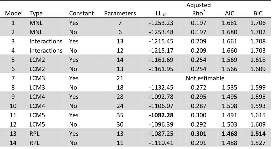
Table 4.3: Summary of Christchurch models
Model Type Constant Parameters LLUR
Adjusted
Rho2 AIC BIC
1 MNL Yes 7 ‐1253.23 0.197 1.681 1.706
2 MNL No 6 ‐1253.48 0.197 1.680 1.702
3 Interactions Yes 13 ‐1215.45 0.209 1.661 1.708
4 Interactions No 12 ‐1215.17 0.209 1.660 1.703
5 LCM2 Yes 14 ‐1161.69 0.254 1.569 1.618
6 LCM2 No 13 ‐1161.95 0.254 1.566 1.609
7 LCM3 Yes 21 Not estimable
8 LCM3 No 18 ‐1132.45 0.272 1.535 1.599
9 LCM4 Yes 28 ‐1092.78 0.295 1.495 1.595
10 LCM4 No 24 ‐1106.07 0.287 1.508 1.593
11 LCM5 Yes 35 ‐1082.28 0.300 1.491 1.615
12 LCM5 No 30 ‐1096.39 0.292 1.503 1.609
13 RPL Yes 13 ‐1087.25 0.301 1.468 1.514 14 RPL No 11 ‐1110.41 0.291 1.488 1.527
LLR = -1564.12 = LL for a model including constants, but no other parameters.
LLUR is the log-likelihood score for the fitted model, whileLLR is log-likelihood for a model
that incorporates only constants, but does not include attributes. One measure of model fit is McFadden’s Rho2. A bigger Rho2 indicates better fit. However, Rho2 cannot be interpreted as the percentage of variance explained (Hensher et al., 2005). Bold cells indicate the model scoring best on each criterion.
Christchurch. For both locations, probability of class membership was not significantly different from zero for at least one class in each of the 5-class models. Minimum BIC is attained at 4 classes in each case. Consequently the 4-class models are adopted as the best LCM alternatives. Significance of group membership is also reported for Latent Class models. Statistically, there is little to choose between the 4-class LCMs and the RPL models.
Overall, there was little difference between models with and without alternative-specific constants. However, in most cases constant terms were not statistically significant. For example, the Christchurch RPL model with a constant (Model 13) was the best-fitting model estimated for Christchurch. However, the constant was far from being statistically significant. Consequently, models without constants are used for subsequent analysis.
Membership of an environmental organisation significantly reduced the probability of membership of Class 1 for Christchurch. LCM models with class membership variables had inferior AIC and BIC scores to the simple LCM models, consequently only models without class membership attributes are reported. Similarly, tests were made of attributes contributing to heterogeneity in the RPL models. Some of these were significant (e.g. male was a determinant of the location of the Stings coefficient), but they did not enhance statistical fit after adjusting for the additional parameters. What is more, they had no detectable effect on estimated willingness to pay.
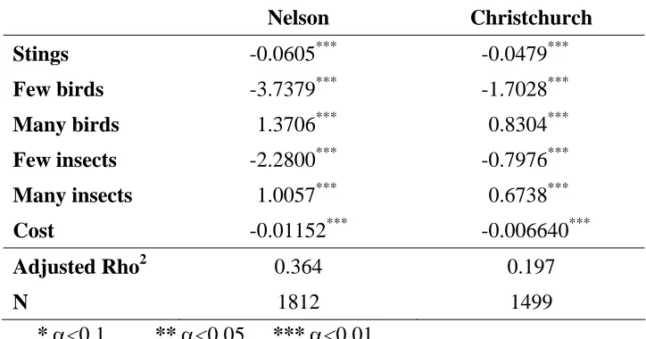
Table 4.4: Multinomial logit models
Nelson Christchurch
Stings -0.0605*** -0.0479***
Few birds -3.7379*** -1.7028***
Many birds 1.3706*** 0.8304***
Few insects -2.2800*** -0.7976***
Many insects 1.0057*** 0.6738***
Cost -0.01152*** -0.006640***
Adjusted Rho2 0.364 0.197
N 1812 1499
* α<0.1 ** α<0.05 *** α<0.01
The variables are:
Stings Probability of being stung on any one summer/autumn day (%) Few birds 1 if there are very few native birds, else 0
Many birds 1 if there are many native birds, else 0 Few insects 1 if there are very few insects, else 0 Many insects 1 if there are many insects, else 0
Cost Annual cost to the household for 5 years ($)
The constant term was not significant in the multinomial logit model for either Nelson or Christchurch. Hence, Table 4.4 reports multinomial logit models that exclude constants. The Rho2 scores approximate R2 in linear regression of about 0.47 (Rho2 = 0.2; Christchurch) to 0.72 (Rho2 = 0.36; Nelson), based on the equivalences reported in Hensher at al. (2005). The Nelson model is an exceptionally good fit for this type of data.
Every attribute in the multinomial logit models is highly significant, and signs on attributes are the same, irrespective of location. Preferences are for fewer stings, more birds, more insects and lower costs, consistent with prior expectations identified in focus groups and during pretesting.
Tables 4.5 to 4.8 present results from models that extend the multinomial logit model in order to accommodate heterogeneity. All offer better statistical fits to the data than the simple multinomial logit models.
Table 4.5: Interactions and latent class models, Nelson
Interactions LCM
Class1
LCM Class2
LCM Class3
LCM Class4 Stings -0.0800*** -0.1155*** -0.0775*** -0.0683*** -0.0088
Male 0.0286***
Few Birds -5.0818*** -34.0727 -2.7400*** -3.3510*** -2.8939***
Male 3.4675***
> 60 years 3.0661***
> $30,000pa -2.0893***
No kids -2.5126**
Many Birds 1.2325*** 2.2153*** 3.7631*** 0.6874*** 2.8068***
Male 0.4067**
Few Insects -2.6294*** -4.8217*** -1.2466*** -1.4411*** -36.9367
No kids -0.9069**
Male 0.7518***
Many Insects 1.2574*** 2.3023*** 0.7035*** 0.3062*** 2.5295***
Male -0.3916**
Cost -0.01212*** -0.01552*** -0.01552*** -0.01552*** -0.01552***
Class Prob. 0.4068*** 0.1160*** 0.3706*** 0.1066***
Adjusted Rho2 0.390 0.449
AIC 1.163 1.059
BIC 1.210 1.132
Table 4.6: Nelson RPL model
Mean SD
Stings -0.09246*** 0.09804***
Few birds -9.6288*** 11.3048***
Many birds 1.9245*** 3.3254***
Few insects -3.9238*** 5.4636***
Many insects 1.4457*** 3.4816***
Cost -0.01622***
Adjusted Rho2 0.438
AIC 1.069
BIC 1.102
* α<0.1 ** α<0.05 *** α<0.01
The Nelson interactions model (Table 4.5) indicates that 4 different personal attributes (Sex, Age, Income, Children in the household) influence estimated parameters. Sex influences all attribute values, with males placing higher value than females on increased bird numbers and also on reduced insect numbers. Males were less concerned than females about increased frequency of stings, reductions in bird or insect numbers, or increased insect numbers. The presence of heterogeneity is further underlined by the LCM coefficients. Few Birds is not significant for Class 1, while Few Insects is not significant for Class 4.
Differences in coefficients indicate different relative importance of attributes for different groups. For example, while Classes 2 and 3 positively and significantly value increases in insect populations, the value of increases in insect populations for Classes 1 and 4 are much higher. Values of reduced bird numbers are similar for all Classes except Class 1. Class 4 places relatively low value on stings, Class 3 values increased bird numbers less than other classes do, and Class 1 places relatively high value on increased insect numbers.
Inclusion of class membership variables in the Latent Class Model offered minor improvements to model fit (Adjusted Rho2 = 0.456, AIC = 1.050, BIC = 1.141). Membership of Class 1 was less likely for males (p = 0.034) and respondents from larger households were more likely to be members of Class 2 (p = 0.084).
The random parameters logit model provides an additional test of heterogeneity. In the Nelson models (Table 4.6) standard deviations of the random parameters are all highly significant and are larger than the means, indicating significant respondent heterogeneity.
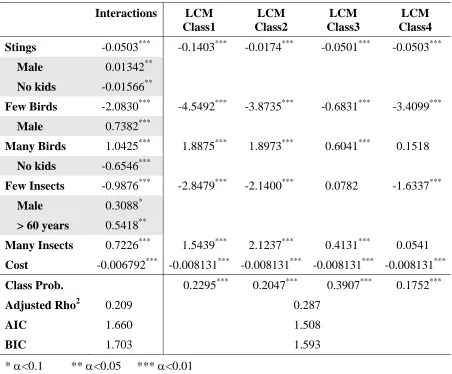
Table 4.7: Interactions and latent class models, Christchurch
Interactions LCM
Class1
LCM Class2
LCM Class3
LCM Class4 Stings -0.0503*** -0.1403*** -0.0174*** -0.0501*** -0.0503***
Male 0.01342**
No kids -0.01566**
Few Birds -2.0830*** -4.5492*** -3.8735*** -0.6831*** -3.4099***
Male 0.7382***
Many Birds 1.0425*** 1.8875*** 1.8973*** 0.6041*** 0.1518
No kids -0.6546***
Few Insects -0.9876*** -2.8479*** -2.1400*** 0.0782 -1.6337***
Male 0.3088*
> 60 years 0.5418**
Many Insects 0.7226*** 1.5439*** 2.1237*** 0.4131*** 0.0541
Cost -0.006792*** -0.008131*** -0.008131*** -0.008131*** -0.008131***
Class Prob. 0.2295*** 0.2047*** 0.3907*** 0.1752***
Adjusted Rho2 0.209 0.287
AIC 1.660 1.508
BIC 1.703 1.593
* α<0.1 ** α<0.05 *** α<0.01
Table 4.8: Christchurch RPL model
Mean Spread
Stings -0.07621*** 0.1349***
Few birds -3.0929*** 4.5300***
Many birds 1.1040*** 2.7198***
Few insects -1.5722*** 3.9558***
Many insects 0.9255*** 2.4304***
Cost -0.009170***
Adjusted Rho2 0.291
AIC 1.488
BIC 1.527
* α<0.1 ** α<0.05 *** α<0.01
Christchurch RPL variances (Table 4.8) are all larger than the means, even more so than for Nelson. As with Nelson, Sex was a determinant of heterogeneity in the Stings parameter, but did little to influence overall model fit.
4.3
Attribute values
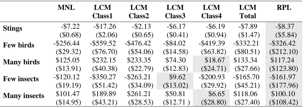
Estimates of willingness to pay and standard deviations are presented in Tables 4.9 and 4.10. The money values estimated for each attribute are derived from the models by dividing the relevant coefficient by the negative of the money coefficient. Because the estimates are ratios of two parameters, each with associated uncertainty, the confidence intervals have been derived using the Delta method (Greene, 2000). Confidence intervals estimated using the Krinsky & Robb method (10,000 replications) provided almost identical standard deviations. Only the Delta method standard deviations are reported here. Because of the complex interactions of numerous different parameters, standard deviations for LCM Total willingness to pay and RPL willingness to pay were derived via Krinsky & Robb (10,000 and 20,000 replicates, respectively). RPL estimates are conditional population measures. Their generally lower level of significance reflects the broad spread of the triangular distribution of the means, which were in the order of one to two times the value of the corresponding parameter mean.
Table 4.9: Willingness to pay, Nelson
MNL LCM
Class1 LCM Class2 LCM Class3 LCM Class4 LCM Total RPL
Stings -$5.25
($0.31) -$7.44 ($0.50) -$4.99 ($0.37) -$4.40 ($0.37) -$0.57 ($0.53) $5.30 ($0.69) -$5.71 ($2.44)
Few birds -$324.59
($26.09)
-$2,196 ($61x106)
-$176.19 ($30.26) -$215.95 ($21.66) -$ 186.49 ($19.97) $1014 ($25x106)
-$586.08 ($288.26)
Many birds $119.02
($8.00) $142.77 ($14.85) $242.51 ($16.63) $44.30 ($7.80) $180.89 ($15.46) $121.91 ($10.66) $118.72 ($84.77)
Few insects -$197.99
($14.14) -$310.73 ($25.77) -$80.34 ($21.18) -$92.87 ($9.76) -$2,380 ($35x107)
$423.87 ($40x106)
-$236.69 ($139.80)
Many insects $87.34
($7.72) $148.37 ($13.62) $45.34 ($14.40) $19.73 ($7.56) $163.01 ($15.28) $90.30 ($11.58) $89.60 ($86.14) (Standard Deviations)
All unshaded cells are significant at the 5% level.
Table 4.10: Willingness to pay, Christchurch
MNL LCM
Class1 LCM Class2 LCM Class3 LCM Class4 LCM Total RPL
Stings -$7.22
($0.68) -$17.26 ($2.06) -$2.13 ($0.65) -$6.17 ($0.41) -$6.19 ($0.94) -$7.89 ($1.47) -$8.37 ($5.84)
Few birds -$256.44
($29.32) -$559.52 ($76.70) -$476.42 ($54.06) -$84.02 ($14.58) -$419.39 ($63.82) -$332.21 ($80.51) -$326.42 ($212.10)
Many birds $125.05
($13.91) $232.15 ($40.38) $233.35 ($22.79) $74.30 ($12.83) $18.67 ($24.71) $133.34 ($27.66) $117.24 ($123.80)
Few insects -$120.12
($19.19) -$350.27 ($51.42) -$263.21 ($34.09) $9.62 ($13.02) -$200.93 ($29.92) -$165.70 ($45.21) -$161.97 ($177.96)
Many insects $101.47
($14.95) $189.89 ($43.21) $261.21 ($28.53) $50.81 ($12.71 ) $6.65 ($28.80) $118.06 ($27.40) $100.10 ($108.42) (Standard Deviations)
Chapter 5
Discussion and Conclusions
Members of the community recruited without any knowledge of the topic of the investigation engaged meaningfully in the choice experiment. They were able to make a series of choices that revealed their preferences about the outcomes of biodiversity management at Nelson Lakes National Park.
The use of schools to recruit community members to participate in group meeting-based surveys again proved highly effective. This process was quick and cheap, yet provided the opportunity to convey high quality background information to participants, and to train them in the choice experiment process in an interactive setting.
Simple statistical models were able to explain a large proportion of the variance in people’s choices. Statistical power was enhanced significantly by the use of models that allowed for respondent heterogeneity. Interactions models that accounted for individual characteristics offered significant, but small, improvements over the basic model. The vastly superior explanatory power of latent class models indicates the existence of distinct groups of preferences within each community. Random Parameters Logit models offered similar explanatory power to Latent Class models. The Latent Class models have the advantage over interactions and Random Parameters models of depicting underlying differences in preferences without the need to parameterise group membership. Hence the Latent Class model accounts for differences in preference structures without being reliant on ascribing those differences to characteristics of the individual. The small improvements in Latent Class model fit by inclusion of class membership variables, but the dramatic improvement of this model over the Interactions model, indicates the stronger role of underlying preferences relative to individual characteristics. The Random Parameters Logit model, while allowing heterogeneity, is poor at predicting community values.
The survey entailed provision of comprehensive information about the distribution, impacts and control of wasps. Consequently, the values reported are not representative of values held now by the community, which has little understanding of wasp impacts or management. Instead, the values reported here reflect the preferences of an informed community, such as might exist subsequent to an open debate about management options for the Lake Rotoiti conservation project.
The samples drawn here were not designed to be representative of each community, or for the selected communities to be representative of the whole of the South Island. However, it is possible to use the results to gain an understanding of the likely magnitude of values for the three attributes included in the study.
Table 5.1: Value estimates
Species Mean annual
value per household
PV @ 10% over 5 years
Aggregate over 300,000 households
Probability of Stings increases by 10%
-$60 -$250 -$75m
Few Birds -$300 -$1250 -$375m
Plentiful Birds $120 $500 $150m
Few Insects -$150 -$625 -$195m
Plentiful Insects $90 $375 $113m
The value estimates derived here, combined with information on the costs of species preservation, whether by managing wasps or other methods, could make an important contribution to cost-benefit analysis of species protection programmes.
References
Bateman, I.J., Carson, R.T., Day, B., Hanemann, M., Hanley, N., Hett, T., Jones-Lee, M., Loomes, G., Mourato, S., Özdemiroglu, E., Pearce, D.W., Sugden, R. and Swanson, J. 2002. Economic valuation with stated preference techniques. Edward Elgar: Cheltenham, U.K.
Beggs, J.R. 1991. Altitudinal Variation in Abundance of common Wasps (Vespula vulgaris). New Zealand Journal of Ecology, 18, 155-158.
Beggs, J., Rees, J.S. and Harris, R.J. 2002. No evidence for establishment of the wasp parasitoid Sphecophaga vesparum burra (Cresson) (Hymenoptera: Ichneumonidae) at two sites in New Zealand. New Zealand Journal of Zoology 29: 205-211.
Beggs, J.R., Toft, R.J., Malham, J.P., Rees, J.S., Tilley, J.A.V., Moller, H. and Alspach, P. 1998. The difficulty of reducing introduced wasp (Vespula vulgaris) populations for conservation gains. New Zealand Journal of Ecology 22(1): 55-63.
Beggs, J.R. and Wardle, D.A. 2006. Keystone Species: Competition for Honeydew Among Exotic and Indigenous Species, Ecological Studies, 186, 281-294.
Bennett, J. and Blamey, R. 2001. The choice modelling approach to environmental valuation. Edward Elgar: Cheltenham, U.K.
Biosecurity NZ undated. http://www.biosecurity.govt.nz/pest-and-disease-response/pests-and-diseases-watchlist/common-wasp.
Champ, P.A., Boyle, K.J. and Brown, T.C. (eds) 2003. A primer on nonmarket valuation. Kluwer: Dordrecht.
Clapperton, B.L., Tilley, J.A.V., Beggs, J.R. and Moller, H. 1994. Changes in the Distribution and Properties of Vespula vulgaris (L.) and Vespula germanica (Fab.) (Hymenopters: Vespidae) Between 1987 and 1990 in New Zealand, New Zealand Journal of Ecology, 21, 295-303.
Ferrini, S. and Scarpa, R. 2007. Designs with a priori information for nonmarket valuation with choice experiments: A Monte Carlo study. Journal of Environmental Economics and Management 53: 342-363.
Greene, W.H. 2000. Econometric analysis, fourth edition. Prentice Hall: New Jersey.
Harris, R.J. 1991. Diet of the wasps Vespula vulgaris and V. germanica in Honeydew beech forest of the South Island, New Zealand. New Zealand Journal of Zoology, 18, 159-170.
Harris, R.J., Moller, H. and Winterbourn, M.J. 1994. Competition for Honeydew Between two social wasps in South Island Beech forests, New Zealand. Insectes Sociaux, 41, 379-394.
24
Hensher, D.A., Rose, J.M. and Greene, W.H. 2005. Applied choice analysis: a primer. Cambridge University Press: Cambridge, U.K.
Kanninen, B.J. (ed.) 2007. Valuing environmental amenities using stated choice studies. Springer: Dordrecht.
Kerr, G.N. and Sharp, B.M.H. 2003. Community mitigation preferences: a choice modelling study of Auckland streams. AERU Research Report No. 256. Agribusiness and Economics Research Unit, Lincoln University.
Kerr, G.N. and Sharp, B.M.H. 2007. The impact of wilding trees on indigenous biodiversity: a choice modelling study. AERU Research Report No. 303. Agribusiness and Economics Research Unit, Lincoln University.
Landcare Research undated. Wasps – Frequently Asked Questions.
http://www.landcareresearch.co.nz/research/bioecons/invertebrates/Wasps/faq.asp.
Louviere, J.J., Hensher, D.A. and Swait, J.D. 2000. Stated choice methods: analysis and application. Cambridge University Press: Cambridge, U.K.
Mainwaring, L. 2001. Biodiversity, biocomplexity, and the economics of genetic dissimilarity, Land Economics, 77(1): 79-93.
Ministry for the Environment. 2007. Protecting our places: information about the statement of national priorities for protecting rare and threatened biodiversity on private land. Ministry for the Environment; Wellington. Available online at www.biodiversity.govt.nz
Mitchell, R.C. and Carson, R.T. 1989. Using surveys to value public goods: the contingent valuation method. Resources for the Future: Washington, D.C.
Navrüd, S. and Ready, R. (eds) 2007. Environmental value transfer: issues and methods. Springer: Dordrecht.
Scarpa, R. and Rose, J.M. 2008. Designs efficiency for non-market valuation with choice modelling: how to measure it, what to report and why. Australian Journal of Agricultural and Resource Economics 52(3): 253-282.
Swait, J.D. 1994. A structural equation model of latent segmentation and product choice for cross-sectional revealed preference choice data. Journal of Retailing and Consumer Services 1(2): 77-89.
Thomas, C.D., Moller, H., Plunkett, G.M. and Harris, R.J. (1990). The prevalence of introduced Vespula vulgaris wasps in a New Zealand beech forest community. New Zealand Journal of Ecology 13: 63-72.
Train, K.E. 1998. Recreation demand models with taste differences over people. Land Economics 74(2): 230-239.
RESEARCH REPORTS
286 The Influence of Perceptions of New Zealand Identity on Attitudes to Biotechnology
Hunt, Lesley and Fairweather, John 2006
287 New Zealander Reactions to the use of
Biotechnology and Nanotechnology in Medicine, Farming and Food
Cook, Andrew and Fairweather, John 2006
288 Forecast of Skills Demand in the High Tech Sector in Canterbury: Phase Two
Dalziel, Paul, Saunders, Caroline and Zellman, Eva 2006
289 Nanotechnology – Ethical and Social Issues: Results from a New Zealand Survey
Cook, Andrew and Fairweather, John 2006
290 Single Farm Payment in the European Union and its Implications on New Zealand Dairy and Beef Trade
Kogler, Klaus 2006
292 Operations at Risk: 2006: Findings from a Survey of Enterprise Risk in Australia and New Zealand
Smallman, Clive 2007
293 Growing Organically? Human Networks and the Quest to Expand Organic Agriculture in New Zealand
Reider, Rebecca 2007
294 EU Positions in WTO Impact on the EU, New Zealand and Australian Livestock Sectors
Santiago Albuquerque, J.D. and Saunders, C.S. 2007
295 Why do Some of the Public Reject Novel Scientific Technologies? A synthesis of Results from the Fate of Biotechnology Research Programme
Fairweather, John, Campbell, Hugh, Hunt, Lesley, and Cook, Andrew 2007
296 Preliminary Economic Evaluation of Biopharming in New Zealand
Kaye-Blake, W., Saunders, C. and Ferguson, L. 2007
297 Comparative Energy and Greenhouse Gas Emissions of New Zealand’s and the UK’s Dairy Industry
Saunders, Caroline and Barber, Andrew 2007
298 Amenity Values of Spring Fed Streams and Rivers in Canterbury, New Zealand: A Methodological Exploration
Kerr, Geoffrey N. and Swaffield, Simon R. 2007
299 Air Freight Transport of Fresh Fruit and Vegetables
Saunders, Caroline and Hayes, Peter 2007
300 Rural Population and Farm Labour Change
Mulet-Marquis, Stephanie and Fairweather, John R. 2008
301 New Zealand Farm Structure Change and Intensification
Mulet-Marquis, Stephanie and Fairweather, John R. 2008
302 A Bioeconomic Model of Californian Thistle in New Zealand Sheep Farming
Kaye-Blake, W. and Bhubaneswor, D. 2008
303 The Impact of Wilding Trees on Indigenous Biodiversity: A Choice Modelling Study
Kerr, Geoffrey N. and Sharp, Basil M.H. 2007
304 Cultural Models of GE Agriculture in the United States (Georgia) and New Zealand (Cantrebury)
Rinne, Tiffany 2008
305 Farmer Level Marketing: Case Studies in the South Island, of New Zealand
Bowmar,Ross K. 2008
306 The Socio Economic Status of the South Island High country
Greer, Glen 2008
307 Potential Impacts of Biopharming on New Zealand: Results from the Lincoln Trade and Environment Model
Kaye-Blake, William, Saunders, Caroline, de Arãgao Pereira, Mariana 2008
308 In progress
309 Public Opinion on Freshwater Issues and Management in Canterbury
Cook, Andrew 2008
DISCUSSION PAPER
145 Papers Presented at the 4th Annual Conference of the NZ Agricultural Economics Society. Blenheim 1997
146 Papers Presented at the 5th Annual Conference of the NZ Agricultural Economics Society. Blenheim 1998
147 Papers Presented at the 6th Annual Conference of the NZ Agricultural Economics Society. Blenheim 2000
148 Papers Presented at the 7th Annual Conference of the NZ Agricultural Economics Society. Blenheim 2001
149 Papers Presented at the 8th Annual Conference of the NZ Agricultural Economics Society. Blenheim 2002
150 Papers Presented at the 9th Annual Conference of the NZ Agricultural Economics Society. Blenheim 2003
151 Papers Presented at the 10th Annual Conference of the NZ Agricultural Economics Society. Blenheim 2004