STATISTICAL VERIFICATION OF
PERFORMANCE OF GENETIC
ALGORITHM IN SCHEDULING
S. G. BHATWADEKAR *
Asst. Professor, Department of Prod. Engg., KIT’s College of Engg., Kolhapur.
M. Y. KHIRE
Professor, Department of Mech. Engg. Dr. PVP College of Engg., Ahmednagar.
Abstract:
Job shop scheduling problem (JSSP) is one of the most researched problem in the area of scheduling. Enumerative solution procedures being computationally ineffective, the research is directed frequently on search methods. Genetic algorithms (GA) provide a powerful search technique with parallel processing of a large number of solutions, while coding the parameters instead of working on the parameters directly. The search is random due to the probabilistic transition rules. The GA operators encourage production of stronger children through the mating of stronger parents as the solution moves through generations. Crossover ensures exploitation while mutation ensures exploration of the solution space without a complete enumeration. In this study ten problem instances of a five-jobs-five-machine JSSP are solved for different combinations of population sizes and number of generations. The results are then analysed for statistical verification of the performance of the GA. The inferences are presented at the conclusion.
Keywords: Genetic algorithm; job shop scheduling; makespan
1. Introduction
Scheduling problems deal with allocation of limited resources over time to perform tasks to satisfy certain objectives. In a job shop scheduling problem (JSSP) we have a set of jobs and a set of machines. Each machine can handle at most one job at a time. Each job consists of a sequence of operations. Further each operation needs to be performed during an uninterrupted time period of known duration on a given machine. The purpose of a JSSP is to find a schedule, that is, allocation of operations to time intervals, with the minimum duration to complete all jobs [Baker, (1974)]. This problem is one of the best known of the difficult combination optimization problems. The number of possible schedules will be excessive, that is about (n!)m, where n is number of jobs and m is number of machines. To find the optimum schedule will consume excessive computational time, sometimes rendering it impossible [Geyik and Cedimoglu, (2004)]. Such problems which do not have an efficient algorithm are called as non-deterministic polynomial hard (NP-hard) problems [Pinedo and Chao, (1999)]. Even for a moderately sized problem involving six jobs and five machines, the number of semi-active schedules will be about (6!)5 or 1.93 x 10¹⁴. It is very much unlikely that adequate computer time will be available for the managers to solve a problem of this size by exhaustive enumeration [Conway et al., (2003)]. Hence mathematical programming or analytical methods have a limited utility in solving JSS problems [Bagchi, (1999)]. The genetic algorithms (GA) serve as a powerful search procedureas they can sample a large search space randomly and efficiently.
1.1.Literature Survey
Genetic Algorithms are powerful and broadly applicable stochastic search and optimization techniques. They have five basic components according to [Gen and Cheng, (2000)]. These are,
a) A genetic representation of solutions to the problem b) A way to create initial population of solutions
c) An evolution function rating solutions in terms of their fitness.
GAs have been used in a wide variety of optimization tasks including combinatorial optimization problems like job shop scheduling [Mitchell, (2002)]. GAs are different than traditional methods in the following ways [Goldberg, (1989)].
GAs work with a coding of a parameter set, not the parameters themselves. GAs search from a population of points, not a single point.
GAs use objective function information, not derivatives or other auxiliary knowledge. GAs use probabilistic transition rules, not deterministic rules.
The main concept behind the theory of GAs is schemata- subsets of the search space defined by same values of the some of the genes in the chromosome. A chromosome can be seen as a vector (a point) in a multidimensional search space, where each gene represents a dimension (axis) and each value of a gene (allele) a coordinate along this dimension. Thus a schema is a hyper plane in the search place. Schemata containing good points statistically score well when sampled. Each point (chromosome) represents a sample of the numerous hyper planes that contain it [Faulkeneur and Bouffouix, (1991)]. Fang et al. (1993) have described a GA approach which produces reasonably good results quickly on standard JSS benchmark problems. Yamada and Nakano, (1997) have discussed the application of GAs to JSS benchmark problems of larger sizes, while proposing a multi-step crossover fusion. Bierworth and Mattfield, (1999) have presented a genetic algorithm which solves the job shop scheduling problem. This algorithm is tested in a dynamic environment under different workload situations. Thereby, a highly efficient decoding procedure is proposed which strongly improves the quality of schedules. Wang and Brunn, (2000) have presented an effective GA for JSSP. The encoding scheme consists of n sub-chromosomes based on loading of each of the n machines. Each one of them consists of m genes representing the job numbers and their processing routines of m operations. A sequence extracted crossover and neighbourhood mutation have been used as the GA operators. The performance of a GA depends on the problem type also. This is because the representation of solutions (chromosomes) and the parameters with their settings depend greatly on the nature of the problem. The need for encoding the JSSP schedule in a legal way in a chromosome has also been emphasized by researchers [Al Hakim, (2001)].
2. Methodology
2.1.Assumptions
Following assumptions are made for the JSS problem. (i) Each operation of a job takes a fixed amount of time.
(ii) Each job has a pre-determined processing sequence and a processing operation once started cannot be interrupted or discontinued before completing.
(iii) At a given time a machine processes only one job. 2.2.Formulation
The problem is formulated as a genetic algorithm with the chromosomes represented as the operation wise sequence of jobs [Al Hakim, (2001)]. The chromosome is partitioned into m number of sub-chromosomes, each representing a job order to be followed for each of the operations. For example, a typical chromosome (schedule) of a five jobs and five machines problem will be described as shown in Table 1.
Table 1: Representation of a schedule in the form of a chromosome
Order of jobs to be followed 1 5 4 2 3 2 1 3 5 4 2 3 5 1 4 5 3 1 4 2 4 5 3 1 2
Processing stage -Operation No. 1 2 3 4 5
The schedule according to this sequence will be prepared for loading the jobs on the machines and the start times and completion times for each operation of all the jobs are calculated. The Fitness Function seeks to minimize the makespan of the schedule. This is the time elapsed between the commencement of the first job and the completion of the last job. Thus the algorithm seeks to minimize the makespan. The initial population of n
chromosomes is created by randomly generating the sequences of job numbers for each operation separately and combining them in the above manner. The chromosomes (schedules) are then evaluated for the makespan. 2.3.GA Operators
The GA operators are applied as described below.
(i) Selection: The chromosomes for the next generation are selected by using the roulette wheel method [Goldberg, (1989)]. This involves calculating the fitness value of each chromosome as follows. The maximum fitness refers to minimum makespan. The fitness of chromosome j is,
Probability of selection of chromosome j, pj = (Fitness)j / ∑( Fitness values)
A random number, r, is generated. If it falls within the cumulative probability values of chromosome j-1
and chromosome j, then chromosome j is selected as a member of the next generation. This is repeated n
times to select total n chromosomes for the next generation. Thus a population of stronger chromosomes is generated for the next iteration.
(ii) Crossover: Crossover is a recombination operator. It recombines in a random manner the partial schedules to create new schedules. The sequences for a randomly selected operation level are interchanged between two randomly selected chromosomes in the mating pool. Suppose Figure 1 shows the two randomly selected chromosomes and further the randomly selected crossover site is 3. Then the new chromosomes will be created as shown in Figure 1.
Old Chromosomes (Parents) New Chromosomes (Children) 1 5 4 2 3 2 1 3 5 4 2 3 5 1 4 5 3 1 4 2 4 5 3 1 2 1 5 4 2 3 2 1 3 5 4 5 1 2 3 4 5 3 1 4 2 4 5 3 1 2
2 1 4 3 5 4 5 3 1 2 5 1 2 3 4 3 4 1 2 5 3 1 5 4 2 2 1 4 3 5 4 5 3 1 2 2 3 5 1 4 3 4 1 2 5 3 1 5 4 2
Figure 1: Crossover Operation
The operation sequence of each job remains legal after crossover by this method [Al Hakim, (2001)]. In this case the crossover probability is chosen as 0.8. Crossover is applied to a generation if a random number between 0 and 1 selected in that generation is less than the crossover probability. A higher value of crossover probability encourages exploitation of the stronger partial schedules.
(iii) Mutation: This operator involves alteration of a single chromosome randomly chosen against a chosen probability. It explores the solution space to find the chance variations. The probability is chosen as 0.1 as a higher value will lead to unstable population and delayed convergence. The mutation applied here inverts the sequence of jobs in a randomly chosen chromosome at a randomly chosen operation level. The occasional mutations insure that useful genes not present in the current population get a chance to enter the population pool [Faulkener and Bouffouix, (1991)].
(iv) Elitist Strategy: There is a possibility that some good solutions may be lost while applying the crossover and mutation operators. Hence to protect them, the best solution from the previous iteration, if lost in the iteration process, is introduced again by replacing the worst solution from the population in the new generation [Mitchell, (2002)].
(v) The Population Size: The population sizes chosen for various runs are 15, 20 and 25 chromosomes. (vi) The Number of Generations: These are chosen as 25, 30, 35, 40, 45 and 50 for different runs.
3. Results and Discussions
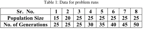
Ten instances offive jobs and five machines (JSS) benchmark problems are taken from [Taillard, (1993)] for this exercise. The proposed algorithm is tested using a program developed in C++ on Windows platform. For each of the combinations shown in Table 1 the problem is solved three times.
Table 1: Data for problem runs
Sr. No. 1 2 3 4 5 6 7 8
Population Size 15 20 25 25 25 25 25 25 No. of Generations 25 25 25 30 35 40 45 50
Table 2: No of occurrences after solving 24 runs of each of the ten problem instances
Prob. Inst.
Makespan Mean Makespan Std. Deviation of
Mean Makespan
Convergence Index
Generations for Convergence
Max Min Decreases Does
not decrease
Converges Diverges near
‘zero’ near
‘one’ Min Max
Ave rage
P1 756 486 24 0 24 0 17 7 3 37 11.5
P2 502 349 24 0 23 1 21 3 5 33 12.1
P3 1066 558 24 0 22 2 20 4 4 31 12.6
P4 584 486 23 1 18 6 18 6 4 42 12.9
P5 658 440 24 0 23 1 21 3 4 39 13.3
P6 690 478 24 0 24 0 19 5 4 33 15.1
P7 808 493 24 0 23 1 18 6 3 38 17.4
P8 475 392 23 1 22 2 20 4 3 26 12.1
P9 592 502 22 2 19 5 19 5 6 37 18.3
P10 689 480 23 1 21 3 21 3 3 30 16.3
Total 235 5 219 21 194 46 - - -
3.1.Statistical analysis
The results are analysed to test the capability of the algorithm first (i) to improve the solution and next to (ii) verify that the solution converges to a better value.
The sample graph of mean makespan plotted against generation number (Figure 2) depicts the capability of improving the makespan. The mean makespan is higher at the initial generations and steadily decreases close to the minimum value towards the final generations. This is observed in about 98 % cases out of the total 240 cases (Table 2). Due to the introduction of new chromosomes in subsequent generations, the mean makespan value shows dispersion through the generations. However this dispersion also narrows down over the generations in 91% of the cases. (Figure 3 and Table 2)
It is necessary that the solution converges in the later generations to a near optimum value. To be able to evaluate the convergence phenomenon a “Convergence Index” of the makespan is defined as follows.
Convergence Index = (Median – Minimum) / (Maximum – Minimum)
When this value is equal to unity, it indicates that at least 50% of the makespan values are equal to the maximum makespan value in that iteration. When the value is equal to zero, it implies that at least 50% of the makespan values are equal to the minimum makespan value in that iteration. Thus as the value of this index approaches zero it is an indication that the solution is converging to the minimum makespan value. A graph in Figure 4 shows the trend of the convergence index against the number of generations in
Figure 2: Mean Makespan vs. Generation No.
490
510
530
550
570
1
6
11 16 21 26 31 36
P9 Gen 40 n25 Gen. No.
Mean Makespan
Figure 3: Dispersion of Mean Makespan vs. Generation No.
Figure 4: Convergence Index Vs. Generation No.
an iteration. The trend shows that the convergence index approaches zero as the generations progress. Table 2 shows the number of cases where the convergence index approaches zero in the total 240 cases. It can be clearly seen that the solution converges to the minimum value in about 80 % of the cases.
Further, the average number of generations required for convergence for the various problem instances ranges from 11 to 18. There are certain cases of earlier or premature convergence too. Premature convergence limits the size of search space and affects the exploration. However the maximum number of generations for convergence (26 to 42) indicates sufficient exploration of the search space.
3.2.Discussions
It is clear from the above exercise that the GAs are capable of finding a workable near-optimum solution to JSS problems in a finite number of generations. In real life situations the practising managers have less inclination to find an optimal solution. A workable near-optimal solution is preferred due to the urgency and frequency of implementation. However this does not undermine the need to reach the optimum or to reach closer to the optimum than the present.
4. Future Scope
Clearly, GAs are not searching the solution space exhaustively. Various approaches are possible for making the solution better.
(i) Mitchell (2002) has suggested that different amounts of selection pressure are needed at different times in a run. For example, in the earlier part lesser fit individuals may be allowed to reproduce at close to the rate of fitter individuals. Thus selection occurs slowly while maintaining a lot of variation in the population ensuring a stronger exploration of the solution space. Later, the highly fit individuals are encouraged more to reproduce. Thus a strong exploration initially and exploitation at later stage can result into a better solution avoiding
0
20
40
60
1
6
11
16
21
26
31
36
P9 Gen40 n25 Gen. No.
Standard Deviation of Mean Makespan
Run 1
Run 2
Run 3
0
0.2
0.4
0.6
0.8
1
1
6
11
16
21
26
31
36
P9 Gen40 n25 Gen. No.
Convergence Index
premature convergence. The Boltzman weighted selection method [Maza and Tidor, (1991)] is an effective way of achieving this result.
(ii) The effectiveness of the GA depends upon the representation of the schedule used. In this study the representation used may pose certain obstacles in reaching nearer to the optimum. The reason is, unless all the jobs are scheduled for the first operation there is no consideration given to the loading of a job for its second operation even though the job is free and the next machine required is also available. This adds to the idle time unnecessarily, thus increasing the makespan and hampering the machine utilization. It is felt that an operation based representation [Bagchi, (1999) and Reddy and Chetty, (2004)] will help in removing this obstacle to a great extent as the algorithm does not wait to complete one operation of all the jobs before loading of the next
operation of any job. However provision to maintain the legality of the schedule after application of the crossover operator has to be incorporated.
(iii) The GA can be combined with a suitable heuristic to strengthen its capability to improve the solution. The examples are Shifting Bottleneck heuristic [Gavereshki, (2008)] or the Giffler Thompson algorithm [Peng et al, (2006)].
(iv) Instead of using GAs alone, they can be supplemented using other search algorithms after reaching a certain level of convergence. The examples are Artificial Neural Networks [(Jain and Meeran, 1998)], Ant Colony Optimisation Algorithm [(Chong et al, 2006)], Particle Swarm algorithm [(Kong et al, 2008)] etc. 5. Conclusion
Genetic algorithms have gained more attention and have been applied to solve combinatorial optimization problems like job shop scheduling. The selection of appropriate representation scheme and the selection operator can help in obtaining a near-optimal solution. Combining the GA with heuristics and use of hybrid algorithms add to the efficacy of the GA implementation.
6. Acknowledgement
The corresponding author is grateful to his parent organization for the necessary support and encouragement for this study which is a part of his Ph. D. related work. The authors also wish to thank their colleagues for the necessary help extended during this exercise.
7. References
[1] Al-Hakim, Latif, (2001), An analog genetic algorithm for solving job-shop scheduling problems”, International Journal of Production Research, 39, 7, pp.1537-1548.
[2] Bagchi, Tapan A., (1999), Multi-objective Scheduling by Genetic Algorithm, Kluwer Academic Publishers, Boston. [3] Baker, K.R., (1974), Introduction to Sequencing and Scheduling, Wiley, New York.
[4] Bierworth, Christain and Mattfield, Dirk C., (1999), Production scheduling and rescheduling with genetic algorithms, Evolutionary Computing,, 7, 1, pp.1-17.
[5] Chong, Chin Soon; Low, Malcolm Yoke Hean; Sivakumar, Appa Iyer and Gay, Kheng, Leng,, (2006), A Bee Colony Optimization Algorithm to Job Shop Scheduling, Proceedings of the IEEE 2006 Winter Simulation Conference, pp.1954-1961.
[6] Conway, Richard W.; Maxwell William W. and Miller, Louis W., (2003), Theory of Scheduling, Dover Publications, New York. [7] Faulkner E. and Bouffouix S., (1991), A genetic algorithm for job shop, Proceedings of 1991 IEEE International Conference on
Robotics and Automation, 824-829.
[8] Fang, Hsiao-Lan; Ross, Peter and Corne, Dave, (1994), A promising hybrid GA / heuristic approach for open shop scheduling problem, Proceedings of 11th European Conference on Artificial Intelligence, pp. 589-594.
[9] Gavereshki, M.H. Karimi and Zarandi, M.H. Fazel, (2008), A heuristic approach for job shop scheduling problems, Journal of Applied Sciences, 8, 6, pp. 992-999.
[10] Gen, Mitsuo and Cheng, Runwei, (2000), Genetic Algorithms and Engineering Optimization, John Wiley and Sons, New York. [11] Geyik, Faruk & Cedimoglu, Ismail Hakki, (2004), The Strategy and Parameters of Tabu Search for Job-shop Scheduling, Journal of
Intelligent Manufacturing., 15, pp. 439-448.
[12] Goldberg, David E., (2001), Genetic Algorithms in Search, Optimization and Machine Learning, Pearson Education, Delhi.
[13] Jain, A.S. & Meeran, S., (1998), Job-shop scheduling using neural networks, International Journal of Production Research, 36, 5, pp. 1249-1272.
[14] Kong, Xiaohong ; Sun, Jun and Xu, Wenbo, (2008), Permutation-based Particle Swarm Algorithm for Tasks Scheduling in Heterogeneous systems with Communication Delays, International Journal of Computational Intelligence Research, 4, 1, pp. 61–70. [15] Maza, Michael de la and Tidor, Bruce, (1991), Boltzmann Weighted Selection Improves Performance of Genetic Algorithms, A.I.
Memo No. 1345, M.I.T. A. I. Laboratory, pp.1-18.
[16] Mitchell, Melanie, (2002), An Introduction to Genetic Algorithms, Prentice Hall of India, New Delhi.
[17] Peng, Lee Hui & Salim, Sutinah, (2006), A modified Giffler and Thompson genetic algorithm on the job shop scheduling problem, MATEMATIKA, 22, 2, pp. 91-107.
[18] Pinedo, M. & Chao, X., (1999), Operations Scheduling with Applications in Manufacturing and Services, Irwin/McGraw Hill, Singapore.
[19] Reddy, M.S. & Chetty, O.V.K., (2004), A genetic algorithm for job shop scheduling, Journal of Institution of Engineers (India) (Production. Division.), 85, pp. 32-35.
[20] Taillard, E., (1993), Benchmarks for basic scheduling problems, European Journal of Operations Research, 64, pp. 278-285.
[21] Yamada, Takeshi and Nakano, Ryohei, (1997), Genetic Algorithms for Job-Shop Scheduling Problems, Proceedings of Conference on Modern Heuristic for Decision Support, UNICOM Seminar, London, pp. 67-81.