https://doi.org/10.5194/nhess-17-971-2017 © Author(s) 2017. This work is distributed under the Creative Commons Attribution 3.0 License.
Sensitivity analysis and calibration of a dynamic physically based
slope stability model
Thomas Zieher1,2, Martin Rutzinger2, Barbara Schneider-Muntau3, Frank Perzl4, David Leidinger5, Herbert Formayer5, and Clemens Geitner1
1Institute of Geography, University of Innsbruck, Innrain 52f, 6020 Innsbruck, Austria
2Institute for Interdisciplinary Mountain Research, Austrian Academy of Sciences, Technikerstraße 21a,
6020 Innsbruck, Austria
3Unit of Geotechnical and Tunnel Engineering, Institute of Infrastructure, University of Innsbruck, Technikerstraße 13,
6020 Innsbruck, Austria
4Austrian Research and Training Centre for Forests, Natural Hazards and Landscape, Rennweg 1,
6020 Innsbruck, Austria
5Institute of Meteorology, University of Natural Resources and Life Sciences Vienna, Peter Jordan Straße 82,
1190 Vienna, Austria
Correspondence to:Thomas Zieher ([email protected]) Received: 13 February 2017 – Discussion started: 16 February 2017 Revised: 29 May 2017 – Accepted: 31 May 2017 – Published: 30 June 2017
Abstract. Physically based modelling of slope stability on a catchment scale is still a challenging task. When apply-ing a physically based model on such a scale (1 : 10 000 to 1 : 50 000), parameters with a high impact on the model result should be calibrated to account for (i) the spatial variability of parameter values, (ii) shortcomings of the selected model, (iii) uncertainties of laboratory tests and field measurements or (iv) parameters that cannot be derived experimentally or measured in the field (e.g. calibration constants). While sys-tematic parameter calibration is a common task in hydro-logical modelling, this is rarely done using physically based slope stability models. In the present study a dynamic, phys-ically based, coupled hydrological–geomechanical slope sta-bility model is calibrated based on a limited number of lab-oratory tests and a detailed multitemporal shallow landslide inventory covering two landslide-triggering rainfall events in the Laternser valley, Vorarlberg (Austria). Sensitive param-eters are identified based on a local one-at-a-time sensitiv-ity analysis. These parameters (hydraulic conductivsensitiv-ity, spe-cific storage, angle of internal friction for effective stress, co-hesion for effective stress) are systematically sampled and calibrated for a landslide-triggering rainfall event in Au-gust 2005. The identified model ensemble, including 25 “be-havioural model runs” with the highest portion of correctly
predicted landslides and non-landslides, is then validated with another landslide-triggering rainfall event in May 1999. The identified model ensemble correctly predicts the loca-tion and the supposed triggering timing of 73.0 % of the ob-served landslides triggered in August 2005 and 91.5 % of the observed landslides triggered in May 1999. Results of the model ensemble driven with raised precipitation input re-veal a slight increase in areas potentially affected by slope failure. At the same time, the peak run-off increases more markedly, suggesting that precipitation intensities during the investigated landslide-triggering rainfall events were already close to or above the soil’s infiltration capacity.
1 Introduction
struc-tures and infrastructure, as well as a loss of agricultural land. To prevent future impacts, it is essential to identify poten-tially affected areas. For this task, various modelling tech-niques are currently applied, including (i) expert-based (e.g. Kienholz, 1977), (ii) statistically based (e.g. Carrara et al., 1991) and (iii) physically based approaches (e.g. Baum et al., 2010). The latter ones are typically based on the limit equi-librium concept and employ physical laws to relate resist-ing to drivresist-ing forces. Their result is a dimensionless factor of safety (FOS), which is a quantitative measure of slope stability. Many physically based approaches include a hy-drological and a geomechanical model element and can be further divided into (i) steady-state (e.g. Dietrich and Mont-gomery, 1998; Montgomery and Dietrich, 1994) and (ii) dy-namic models (e.g. Baum et al., 2010; Crosta and Frattini, 2003). In contrast to steady-state models, dynamic models allow for the spatio-temporal assessment of hillslope hydrol-ogy and stability. Physically based slope stability models can be upscaled to medium scale (1 : 10 000 to 1 : 50 000) using a raster-based geographical information system (GIS). How-ever, such spatially distributed models require data on the spatial distribution of the included parameters (van Westen et al., 2006). To overcome the problem of usually unknown material characteristics throughout the study area, probabilis-tic approaches have proven feasible (Hammond et al., 1992; Raia et al., 2014).
Before applying a spatially distributed physically based model, parameter values are often calibrated to minimize the difference between observations and simulation results. One way of achieving this is to vary the model input parameter values in order to find optimum values or value ranges which yield a general agreement between observations and simula-tions (back calculation). This task is common in hydrologi-cal modelling involving a high-dimensional parameter space (e.g. Dobler and Pappenberger, 2013; Tang et al., 2007). The underlying principles also apply to physically based slope stability models. Theoretically, calibration is not necessary as long as the parameter values are based on a sufficient num-ber of direct measurements or laboratory tests. However, a calibration is advisable (i) if the spatial distribution and vari-ability of parameter values is unknown, (ii) to account for model shortcomings compared to the represented physical processes, (iii) to account for uncertainties of laboratory tests and field measurements or (iv) if parameter values cannot be derived experimentally or measured in the field (e.g. calibra-tion constants). The calibracalibra-tion procedure should be based on physical reasoning and only involve sensitive parameters (i.e. parameters with a distinct impact on the model’s out-come) (Bathurst et al., 2005; Wagener and Kollat, 2007). To identify sensitive parameters, a sensitivity analysis is usually performed. A simple but often applied method is based on the local assessment (one representative raster cell) of the impact of systematic variations of one-parameter-at-a-time (OAT) on the model’s results (e.g. Hammond et al., 1992). This method is also frequently used for parameter value
cali-bration (e.g. Gioia et al., 2016; Salciarini et al., 2006). How-ever, the OAT assessment of parameter sensitivity becomes unreliable with an increasing number of considered param-eters, correlated parameters and non-linear model behaviour (Wagener and Kollat, 2007). As an alternative, global meth-ods which cover the whole parameter space can overcome this drawback (Dobler and Pappenberger, 2013; Tang et al., 2007). Their main disadvantage is the high computational ef-fort, usually requiring a high-performance computing clus-ter (HPCC). Depending on the sampling technique, a mul-titude of parameter value combinations is tested and evalu-ated based on observations. However, instead of identifying a single parameter set which explains the observations best, an ensemble of “behavioural model runs” is often used for the final prediction. These model runs are in general agree-ment with the observations, while their disagreeagree-ment reflects model uncertainty (Bathurst et al., 2005; Wagener and Kol-lat, 2007).
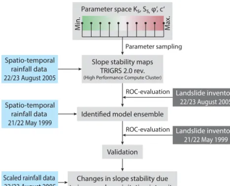
In the present study, the parameters of a revised form of the spatially distributed, dynamic, physically based slope stability model TRIGRS 2.0 (Transient Rainfall Infiltration and Grid-Based Regional Slope-Stability Analysis; Baum et al., 2008, 2010) are systematically tested and calibrated. The four main steps of the analysis are shown in Fig. 1. First, sensitive parameters of the revised model are identi-fied with a local OAT sensitivity analysis. The tested param-eter space is derived from a limited number of laboratory tests and relevant literature. Then, the four identified sensi-tive parameters (hydraulic conductivity, specific storage, an-gle of internal friction for effective stress, cohesion for effec-tive stress) are systematically sampled from a uniform dis-tribution. Unlike in probabilistic parameter sampling strate-gies (e.g. Raia et al., 2014), the parameters are sampled with defined, constant increments. In the calibration procedure, the best 25 “behavioural model runs” are identified out of 10 000 conducted simulations considering each sampled pa-rameter value combination. The ensemble of these 25 model runs optimally predicts the location and the supposed trigger-ing timtrigger-ing of observed shallow landslides, triggered durtrigger-ing a rainfall event in August 2005. The predictive performance of this model ensemble is then tested for another landslide-triggering rainfall event which occurred in May 1999. Fi-nally, the model ensemble is re-run with positively scaled input precipitation maps to give an estimate of potential im-pacts of increasing precipitation intensities on slope stability.
The objectives of the present study are
– to identify sensitive parameters of the revised dynamic physically based slope stability model TRIGRS 2.0; – to present a procedure for a global parameter calibration
Parameter sampling
Min. Max.
Parameter space Ks, Ss, φ‘, c‘
Spatio-temporal rainfall data 22/23 August 2005
Spatio-temporal rainfall data 21/22 May 1999
Scaled rainfall data 22/23 August 2005
Slope stability maps TRIGRS 2.0 rev. (High Performance Compute Cluster)
Identified model ensemble
Landslide inventory 22/23 August 2005 ROC-evaluation
Validation
Landslide inventory 21/22 May 1999 ROC-evaluation
Changes in slope stability due to increased precipitation intensity
Figure 1.Workflow with the main steps of the analysis.
– to evaluate the capability of the identified model ensem-ble for quantifying potential changes in slope stability associated with increasing precipitation intensity.
2 Study area
The study area is located in the Laternser valley in Vorarl-berg, the westernmost province of Austria (Fig. 2a). It covers the catchment area (52.1 km2) of the river Frutz, a tributary of the Rhine. The valley extends about 13 km in the east–west direction, following the strike angle of the Bregenzerwald Mountains. Its highest point is the Hoher Freschen (2004 m) at the head of the valley. The outlet at approximately 500 m is characterized by a steeply incised gorge. In the Laternser valley about half of the catchment area is covered by for-est (2001: 51.0 %; 2006: 50.9 %). A majority of the forfor-est stands are composed of fir (Abies albaMiller) and spruce (Picea abiesL. Karsten), with beech (Fagus sylvaticaL.) oc-curring below 1300 m (Amann et al., 2014). Around 1.2 % of the catchment area is occupied by settlements and infras-tructure. The remaining area is predominantly used as hay meadow or pasture or a combination of both.
2.1 Geology
The Laternser valley is built up by different tectonic units, including a variety of geological units (Fig. 2c, Table 1). Hel-vetic nappes in the western and northern part of the valley in-clude competent limestones (e.g.Schrattenkalk,Seewerkalk) and marls with calcareous layers (e.g. Drusbergschichten). To the south-east, Ultrahelvetic nappes are superimposed, which are mainly built up of clayey marls and shales (e.g.
Leimernmergel). On top in the south-east of the catchment area, Penninic nappes make up more than half of the
val-ley. These nappes include mainly sandstones (e.g. Reisels-berger Sandstein,Planknerbrückenserie) and thinly layered marls (e.g.Piesenkopfschichten) (Friebe, 2007; Heissel et al., 1967; Oberhauser, 1982, 1998). Widespread till deposits and hillside debris cover more than 57 % of the catchment area. These units are overly susceptible to shallow landsliding (Zieher et al., 2016). In numerous cases, subglacial till is re-ported to act as an impermeable layer and slip surface for the unconsolidated material on top. Furthermore, marls of the Ultrahelvetic nappes, as well as less competent sandstones of the Penninic nappes, are particularly susceptible to shal-low landsliding (Zieher et al., 2016).
2.2 Climate
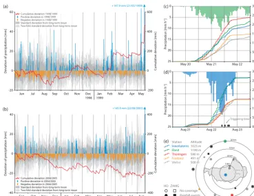
Oceanic air masses advecting from the north-west dominate the warm temperate climate of Vorarlberg. On the Alpine rim in northern Vorarlberg, precipitation amounts are higher due to blocking of the inflowing air masses (Werner and Auer, 2001a, b). Because of the valley’s orientation, it is prone to north and north-westerly weather conditions. At Innerlaterns station (location mapped in Fig. 2c), mean annual precip-itation exceeds 1800 mm a−1 (period 1981–2010). Consid-ering a potential evaporation in Vorarlberg on the order of 600 mm a−1 (Werner and Auer, 2001a), a year-round high amount of seepage water can be assumed.
On the synoptic scale, the landslide-triggering rainfall events in May 1999 and August 2005 occurred in the course of so-called Vb weather situations (van Bebber, 1891; For-mayer and Kromp-Kolb, 2009). Such synoptic meteorologi-cal situations are characterized by a low forming south of the Alps, subsequently moving to the north-east. The moisture taken up over the Mediterranean and Adriatic Sea is trans-ported to eastern-central Europe, potentially causing heavy rainfalls in large parts of Austria (Seibert et al., 2007). 2.3 Landslide-triggering rainfall events
Table 1.Information on the geological units shown in Fig. 2c and their respective lithology (Heissel et al., 1967; Oberhauser, 1958, 1982; Friebe, 2007). Only geological units covering more than 1 % of the catchment area are listed.
Tectonic unit No. Geological unit Lithology Age
Quaternary 1 Hillside debris Unconsolidated materials Quaternary
2 Till deposits Unconsolidated materials Quaternary
Helveticum
3 Globigerinenmergel Calcareous marls Eocene
4 Grünsandstein Sandstones Eocene
5 Seewerkalk Competent limestones Upper Cretaceous 6 Schrattenkalk Competent limestones Lower Cretaceous 7 Drusbergschichten Marls with calcareous layers Lower Cretaceous
Ultrahelveticum 8 Leimernmergel Clayey marls and shales Upper Cretaceous
Penninicum
9 Reiselsberger Sandstein Competent sandstones Upper Cretaceous 10 Piesenkopfschichten Thin-layered limestones Upper Cretaceous 11 Planknerbrückenserie Sandstones Upper Cretaceous
Figure 2.Location of the Laternser valley(a), slope angle map(b), geological map with sampled sites(c)and shallow landslide inventory(d). The slope angle map is based on a digital terrain model derived from airborne laser scanning (ALS) in 2011, serving as input data for modelling (resampled to a spatial resolution of 10 m). The box plots show the slope angle distribution for forest and non-forest areas. In the geological map only geological units covering more than 1 % of the catchment area are listed in the legend (data source: Heissel et al., 1967; Oberhauser, 1982). The shallow landslide inventory shows landslides triggered by the rainfall events in May 1999 (82; yellow) and August 2005 (356; red) occurring on undisturbed hillside slopes (Zieher et al., 2016). The areas covered by forest were derived from ALS data acquired in 2011.
the onset of the landslide-triggering rainfall event on 21–22 May, with a total sum between 134.0 mm at Frastanz station and 212.8 mm at Thüringen station (Fig. 3c).
Monthly precipitation sums from November 2004 to June 2005 generally fell below the long-term mean, except for February and May (Fig. 3b). Therefore it can be expected that no exceptional antecedent soil moisture preceded the rainfall event in August. However, the amount of precipita-tion in July and the first half of August corresponds to the
of the local voluntary fire brigade (Fig. 3d). Most landslides occurred over the course of the night from 22 to 23 August.
3 Materials and methods 3.1 Shallow landslide inventory
A comprehensive shallow landslide inventory was compiled for the catchment area of the Laternser valley, based on the systematic interpretation of nine orthophoto series covering the period from 1950 to 2012 (Zieher et al., 2016). Landslide mapping was aided by digital terrain models (DTMs) de-rived from two airborne laser scanning (ALS) campaigns and their differential digital terrain model (dDTM). In addition, data from two field surveys conducted immediately after two landslide-triggering rainfall events in May 1999 and August 2005 and associated archive data were included in the inven-tory. In total, 82 shallow landslides attributed to the rainfall event in May 1999 and 356 shallow landslides triggered in August 2005 were used for this study (Fig. 2d). Only rainfall-triggered shallow landslides which occurred on undisturbed hillside slopes were considered. They account for three quar-ters of the observed landslides for both rainfall events. Ob-served shallow landslides on other slope types may involve additional causative factors for slope failure, which are not included in the model (e.g. weakened foot slope). Of the con-sidered landslides, 28 (34.1 %; May 1999) and 88 (24.7 %; August 2005) are located within forests.
3.2 TRIGRS 2.0 model
The dynamic, physically based, coupled hydrological– geomechanical model TRIGRS 2.0 was developed by Baum et al. (2008, 2010) and is written in the Fortran program-ming language (USGS, 2016). TRIGRS 2.0 is based on a raster environment and implements a hydrological model el-ement (a run-off model and two types of infiltration models) and a geomechanical model element (infinite slope stability model). It is suitable for modelling the spatio-temporal pro-gression of slope stability in the course of rainfall events with a duration of up to a few days (Baum et al., 2010).
In the model, the infiltration process and associated effects on slope stability are computed dynamically for each raster cell in defined time intervals. Run-offRdis routed downslope
from raster cells where the precipitation intensityP plus the incoming run-offRufrom adjacent raster cells above exceed
the infiltration capacity (equal to the hydraulic conductivity
Ks; Baum et al., 2008):
Rd=
(
P+Ru−Ks ifP+Ru−Ks≥0
0 ifP+Ru−Ks<0.
(1)
However, the amount of run-off is not passed on to the next time interval. The available amount of water ready for infiltration on each raster cell is passed on to the infiltration
model. For tension-saturated initial conditions, a generalized pore pressure diffusion model after Iverson (2000) can be applied. The predictive performance of Iverson’s model has been tested in the Laternser valley on a plot scale (Zieher et al., 2017). For unsaturated conditions, an analytical so-lution for unsaturated flow following Srivastava and Yeh (1991) can be applied. However, the exponential model de-scribing the soil water retention curve (Gardner, 1958) used for linearizing Richard’s equation is considered suitable for coarse-grained materials (Baum et al., 2008) and hence not suitable for the application in the Laternser valley. The de-tails of the infiltration models have been presented in previ-ous studies (e.g. Baum et al., 2010; Iverson, 2000; Kim et al., 2013; Park et al., 2013; Salciarini et al., 2006). The result of both infiltration models is the evolution of pore pressures with depth and time as a response to the infiltration of time-varying precipitation. Pore pressuresψ (d, t )are passed on to the infinite slope stability model relating driving to resisting stresses (FOS):
FOS(d, t )=tanϕ
0
tanβ +
c0−ψ (d, t )·γw·tanϕ0
γs·d·sinβ·cosβ
, (2)
whered (m) is the vertical depth (positive in downward di-rection),t(s) is time,ϕ0(deg) is the angle of internal friction for effective stress,β (deg) is the slope angle,c0(Pa) is the cohesion for effective stress per unit area,γw(9806.6 N m−3)
is the unit weight of water andγs(N m−3) is the unit weight
of soil. Raster cells where the FOS falls below 1.0 are con-sidered slope failures. Each cell with a FOS<1.0 repre-sents a single shallow landslide (Milledge et al., 2012). The model’s results are FOS maps showing a quantitative mea-sure of slope stability in space and time.
However, the original version of TRIGRS 2.0 does not ac-count for effects of vegetation. Kim et al. (2013) extended the model to include vegetation effects on hydrology and slope stability. They conclude that root reinforcement and tree sur-charge can affect slope stability, while interception has only minor effects during landslide-triggering rainfall events. Fol-lowing Kim et al. (2013), lateral root cohesioncr (Pa) and
tree surchargest(Pa) were added to Eq. (2):
FOS(d, t )=tanϕ
0
tanβ +
c0+cr−ψ (d, t )·γw·tanϕ0
(st+γs·d)·sinβ·cosβ
. (3)
Instead of adding a constant value forcr(e.g. Kim et al.,
2013), a linear decrease ofcrwith depth up to a given rooting
depthdr(m) was assumed, accounting for the distribution of
roots with depth as observed in other studies (e.g. Bischetti et al., 2005, 2009). If the rooting depth exceeds the regolith depth,cris only considered down to the regolith–bedrock
in-terface (roots are not expected to penetrate the bedrock). For the revised form of TRIGRS 2.0, three additional parame-ters (cr,st anddr) must be given. The three parameters are
Sep Oct Nov Dec Jan Feb Mar Apr May Jun Jul Aug -40 -20 0 20 40 De
viation of precipitation [mm]
-400 -200 0 200 400 Cum ulativ
e deviation [mm]
2004 2005 Cumulative deviation 2004/2005 Positive deviation in 2004/2005 Negative deviation in 2004/2005 Standard deviation from long-term mean Two-fold standard deviation from long-term mean -20 0 20 40 60 De
viation of precipitation [mm]
-200 0 200 400 600 Cum ulativ
e deviation [mm]
+147.9 mm (21/05/1999)
+145.9 mm (22/08/2005)
Jun Jul Aug Sep Oct Nov Dec Feb Mar Apr May
1998 1999Jan
Cumulative deviation 1998/1999 Positive deviation in 1998/1999 Negative deviation in 1998/1999 Standard deviation from long-term mean Two-fold standard deviation from long-term mean
5 km 10 km 15 km 20 km HD ZAMG No coverage Rainfall events
Long-term mean 00 2 4 km
Altitude 1025 m 1100 m 580 m 491 m 500 m Altitude 1025 m 1100 m 580 m 491 m 500 m Station Innerlaterns Ebnit Thüringen Frastanz Weiler Laternser valley Laternser valley
Aug 21 Aug 22 Aug 23 0
25 300 0 50 100 150 200 250 Cum ulativ
e precipitation [mm]
20 15 10 5
Precipitation [mm h
-1]
Triggering time
May 20 May 21 May 22 0
25 300 0 50 100 150 200 250 Cum ulativ
e precipitation [mm]
20 15 10 5
Precipitation [mm h
-1] (a) (b) (c) (e) (d)
Figure 3.Landslide-triggering rainfall events in the Laternser valley on 21–22 May 1999(a, c)and 22–23 August 2005(b, d). The map(e)
shows the meteorological stations considered. Regional daily mean (07:00–07:00) and cumulative deviation of precipitation from the
long-term mean (1981–2010) are shown for the period of 1 year before the rainfall events(a, b). Cumulative precipitation for 3 days covering
the landslide-triggering rainfall events are shown for meteorological stations within and surrounding the Laternser valley(c, d). Hourly
precipitation sums are shown for Ebnit station in May 1999(c), because at Innerlaterns station missing values are present in the respective
hourly time series. Estimated triggering times of four shallow landslides were derived from protocols by the voluntary fire brigade. Data source: Hydrographic Service of Vorarlberg (HD), Central Institute for Meteorology and Geodynamics (ZAMG).
3.3 Model parameters
Table 2 shows the required parameters and their values con-sidered in previous studies with the original TRIGRS model (versions 1.0 and 2.0) and a revised form (Kim et al., 2013). In the cited studies, the time-varying precipitation intensities are derived from meteorological stations in or near the study area. The slope angle maps are calculated using digital eleva-tion models (based on interpolated contour lines) of various spatial resolutions. Regolith depth maps are prepared as a function of the slope angle (Salciarini et al., 2006), using a geomorphologically indexed model (Zizioli et al., 2013), us-ing a spline interpolation of direct measurements (Kim et al., 2013) and with spatially constant values (Park et al., 2013; Vieira et al., 2010). The initial depth of the water tabledwi
(positive in downward direction) is assumed to be either at the regolith–bedrock interface (Kim et al., 2013; Park et al., 2013; Vieira et al., 2010) or at a depth relative to it (Salciarini et al., 2006; Zizioli et al., 2013). For the background infil-tration rate describing a steady-state infilinfil-tration component, constant values (e.g. Kim et al., 2013; Vieira et al., 2010) or multiples ofKs(e.g. Park et al., 2013) were used.
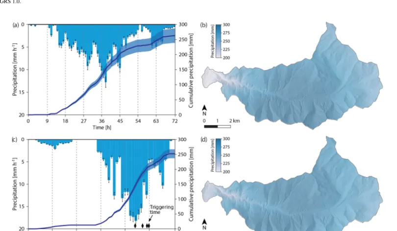
For the landslide-triggering rainfall events considered in the present study, hourly precipitation maps were prepared for the whole province of Vorarlberg. Based on hourly precipitation records from available meteorological stations throughout the province, hourly precipitation maps were gen-erated using a spline interpolation. Figure 4 shows the re-spective time series and the resulting cumulative precipita-tion maps for the Laternser valley. The temporal course of the precipitation intensities differs distinctly (August 2005: short and intense; May 1999: prolonged and less intense), while cumulative precipitation sums over the considered duration are of the same order (May 1999: 263 mm; August 2005: 252 mm). For modelling the temporal evolution of slope stability, FOS maps were computed for nine (May 1999; Fig. 4a) and seven (August 2005; Fig. 4c) time steps with intervals of 9 h to completely cover both rainfall events.
ar-Table 2.Parameters for the revised TRIGRS 2.0 model and parameter values considered in previous studies. DEM: digital elevation model;
Ks: saturated hydraulic conductivity.
Parameter Unit Salciarini et al. (2006) Zizioli et al. (2013) Vieira et al. (2010) Park et al. (2013) Kim et al. (2013)∗ Precipitation intensityP m s−1 Station data Station data Station data Station data Station data
Slope angleβ Degree DEM (5×5 m) DEM (10×10 m) DEM (2×2 m) DEM (10×10 m) DEM (5×5 m)
Regolith depthdmax m Function of Geomorphologically Constant value Constant value Spline interpolation
slope angle indexed model (1.0, 2.0 and 3.0 m) (2.0 m) of measurements
Initial depth of the m 0, 25, 50 and 100 % 0.75 m below At regolith At regolith At regolith
water tabledwi of regolith depth the surface depth depth depth
Background infiltration rateIz m s−1 – – 1.00×10⁻⁹ 0.01×Ks 4.50×10⁻⁹
Angle of internal friction for Degree 18.00–40.00 22.00–33.70 34.00 29.63 34.00
effective stressϕ0
Cohesion for effective stressc0 kPa 4.00–100.00 0.00–10.00 1.00; 6.00 10.17 5.20
Sat. hydraulic conductivityKs m s−1 10−8−10−4 1.50×10⁻⁵−1.00×10⁻⁴ 1.00×10⁻⁶ 1.30×10⁻⁵ 4.50×10⁻⁵
Hydraulic diffusivityD0 m2s−1 – – 5.5×10⁻⁵ 200×Ks –
Unit weight of soilγ kPa 18.00–22.00 17.46–19.91 17.10; 14.30 18.38 14.71
Root cohesioncr kPa – – – – 3.0
Tree surchargest kPa – – – – 2.9
Rooting depthdr m – – – – –
Number of property zones 5 4 1 1 1
∗Revised form of TRIGRS 1.0.
Figure 4.Hourly precipitation time series(a, c)and spatially interpolated precipitation sums(b, d)for the duration of the landslide-triggering
rainfall events in 1999 (a,b; 07:00 on 20 May to 07:00 on 23 May) and 2005 (c,d; 07:00 on 21 August to 12:00 on 23 August). The error
bars and the shading for the cumulative precipitation sum in(a)and(c)indicate the range of the interpolated hourly precipitation sums within
the catchment area.
eas covered by forest. The spatial resolution of the prepared parameter maps was set to 10 m with regard to the most abun-dant size of observed landslide scar areas, which is on the order of 100 m2(Zieher et al., 2016). Furthermore, the cho-sen spatial resolution was considered a compromise between the topographical representation of the surface, the computa-tional efficiency for the modelling and the required minimum length-to-depth ratio (on the order of 8 : 1) for the application of the infinite slope stability model (Milledge et al., 2012).
Figure 5.Cumulative distribution ofdmaxderived from observations and models(a)and the resulting regolith depth map(b).
measurements (e.g. Lanni et al., 2012; Wiegand et al., 2013), (ii) means of geophysics (e.g. Davis and Annan, 1989; Sass, 2007) and (iii) modelling (e.g. Dietrich et al., 1995; Heim-sath et al., 1997). Furthermore, the depth of past landslides can be derived from multitemporal, remotely sensed eleva-tion data (Zieher et al., 2016). For regolith depth mapping, regression models correlating regolith depth to either eleva-tion, slope angle or other derivatives were used in previous case studies on shallow landslide susceptibility (Baum et al., 2010; Lanni et al., 2012; Salciarini et al., 2006; Segoni et al., 2012). For the assessment of regolith depth in the Laternser valley, 126 dynamic cone penetration tests (DCPTs) were conducted along four transects. A lightweight dynamic cone penetrometer with a 10 kg hammer dropped from a height of 0.5 m onto an anvil of 6 kg was used (e.g. Wiegand et al., 2013). Following ÖNORM EN ISO 22476-2:2012, the num-ber of strokes for penetrating vertical increments of 10 cm was recorded in the field. After completing 50 strokes, the penetration tests were stopped if the penetrated increment was less than 10 cm (ÖNORM EN ISO 22476-2:2012). The final depth was recorded to the nearest centimetre, with the maximum detectable depth of 6.0 m exceeded only once. Furthermore, the maximum vertical depths of 96 shallow landslides triggered on 21–22 May 1999 and of 249 shal-low landslides triggered on 22–23 August 2005 are available for validation (Fig. 5b). The landslide depths were measured in the field after the triggering event in May 1999 (Andrecs et al., 2002) and derived from the analysis of a dDTM for the landslides triggered in August 2005 (Zieher et al., 2016). The final depths of the DCPTs were used to train generalized linear models (GLMs) with local morphometric parameters as predictors, including elevation, slope angle, minimum and maximum curvature (Wood, 1996), and the topographic wet-ness index (Beven and Kirkby, 1979). A stepwise backward predictor selection revealed a linear model with the slope an-gle yielding the best agreement with the cumulative landslide depths from 1999 and 2005 (Fig. 5a). It outperforms the cur-vature and the combined slope angle–curcur-vature model, par-ticularly for depths below 2.0 m. The resulting empirical
re-lationship for regolith depthdmaxand the slope angleβis
dmax=
(
3.028−0.049·β for 0.0◦≤β <61.8◦
0.0 forβ≥61.8◦. (4)
The derived regolith depth map (Fig. 5b) also matches the field observation that on slopes which are inclined more than approximately 60◦the surficial cover of unconsolidated ma-terial is of minor depth or not present at all. Furthermore, on very steep slopes there is a transition from sliding to toppling and falling as the predominant types of failures (Baum et al., 2010).
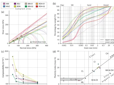
For the derivation of the geotechnical and hydrological pa-rameter values suitable for the Laternser valley, a limited number of laboratory tests were conducted. On the south-facing slopes of the study area, geotechnical samples were collected from eight sites where shallow landslides had been triggered in 1999 (BIN-02), 2002 (ROH-01), 2005 (BIN-01, BON, MAZ, REU, ROH-02) and 2013 (INN), close to popu-lated areas in the Laternser valley (Fig. 2c, Table 3). The ab-breviations were chosen according to the closest settlements (BIN: Bingadels; BON: Bonacker; INN: Innerlaterns; MAZ: Mazona; REU: Reute; ROH: Rohnen). In the geological map (Fig. 2c), the sampled sites are mapped as hillslope debris (BIN-01, BIN-02), till deposits (INN, MAZ, REU, ROH-01),
Leimernmergel (BON) and Drusbergschichten (ROH-02).
Back walls were laid open at the top of the landslide scarps. Two undisturbed and one disturbed sample were taken at two depths at each site except for location ROH-02. There, sam-ples of one depth were considered sufficient because of the homogeneously structured regolith. The undisturbed samples were collected with the help of core cutters (diameter 9.6 cm) and stored airtight. Furthermore, buckets of material were taken from the respective depths. The grain size distributions (Fig. 6b), wet and dry bulk densities and water contents were determined for all samples. With the lower samples, geotech-nical parameters (ϕ0,c0, Atterberg limits) were derived from the respective laboratory tests (Fig. 6a, d). The upper sam-ples were used to obtain estimates for the specific storageSs,
based on the constrained modulusEs(Pa) derived from
val-ues forSs(m−1) were derived from
Ss=ρw·g·(αs+n·βw), (5)
whereρw(kg m−3) is the density of water,gis the
acceler-ation of gravity (9.81 m s−2),nis porosity, βw is the
com-pressibility of water (4.4×10⁻¹⁰m2N−1) andαs (m2N−1)
is the compressibility of bulk soil (Fig. 6c), derived from
αs=
3·(1−v) Es·(1+v)
, (6)
where v is Poisson’s ratio, for which a constant value of 1/3 was assumed (e.g. Lu and Godt, 2013; Schmidt et al., 2014). Es depends on the prevailing stress level (i.e.
over-burden height; Schmidt et al., 2014) and was derived for a depth of 1–2 m (e.g. Berti and Simoni, 2010). The hydraulic diffusivityD0(m2s−1) was derived from
D0=
Ks
Ss
. (7)
However,Ks was not tested in the field or laboratory. Its
parameter values were calibrated over several orders of mag-nitude. The background infiltration rate was set to zero to consider a conservative estimate of pore pressure conditions assuming a slope-parallel groundwater flow (Baum et al., 2008, 2010).
For the parameters representing the effects of vegetation on slope stability in the revised model, spatially constant parameter values are assumed within the area covered by forest. A conservative set of parameter values is derived from respective literature with cr set to 2.5 kPa (e.g.
Bis-chetti et al., 2009; Steinacher et al., 2009),st set to 2.5 kPa
(e.g. Steinacher et al., 2009) and dr set to 1.0 m (e.g.
Bis-chetti et al., 2009; Kutschera and Lichtenegger, 2002). How-ever, these values were only applied within areas covered by forest. A forest cover map was prepared, based on the normalized digital surface model (nDSM) derived from the ALS data from 2011. The areas covered by forest for the time of the two landslide-triggering rainfall events in Au-gust 2005 and May 1999 was adapted manually, using high-resolution orthophotos from 2006 (ground sampling distance of 0.125 m) and 2001 (ground sampling distance of 0.25 m) respectively.
3.4 One-parameter-at-a-time sensitivity analysis Following Hammond et al. (1992), the model’s sensitivity against each parameter is tested individually. For each pa-rameter, central, minimum and maximum values are defined based on laboratory tests, field investigations and respective literature (Table 4). The resulting FOSpi for each parameter pi sampled over the specified range is related to the
respec-tive FOSpcentralbased on the defined central parameter values:
1FOS=FOSpi−FOSpcentral
FOSpcentral
. (8)
The resulting relative deviation1FOS reflects the model’s sensitivity against each parameter. However, interactions be-tween parameters are not considered (Dobler and Pappen-berger, 2013; Hammond et al., 1992).
3.5 Parameter calibration and validation
In previous studies, local OAT parameter tests were used for the calibration of parameter values (e.g. Gioia et al., 2016). In the present study, the calibration of the four identified sensi-tive parameters (ϕ0,c0,Ks,Ss; Sect. 4.1) is based on
system-atic testing of parameter value combinations for the whole catchment area (global calibration), computed with a HPCC (162 nodes, 1.944 Intel Xeon Gulftown compute cores). For each parameter, 10 values are sampled from a uniform dis-tribution in equal increments from the defined minimum to maximum (e.g. Beven and Freer, 2001). Because of the lim-ited number of laboratory tests, it is not possible to infer probability distributions of the parameter values. The hydro-logical parameters are sampled on the logarithmic scale (Ta-ble 5).
The predictive performance of each FOS map resulting from the 10 000 calibration runs with seven time steps each (514.9 GB of data) was assessed with the receiver operat-ing characteristic (ROC) principle (Begueria, 2006). Usoperat-ing physically based slope stability models, a FOS<1.0 indi-cates a potential slope failure, while a FOS≥1.0 suggests a stable slope. The coordinates of the point in the ROC plot where the FOS falls below 1.0 represent the correctly pre-dicted fractions of observed landslides (true positives; TP) and non-landslides (true negatives; TN). The basic idea of the calibration procedure is to identify parameter value com-binations which result in an optimum prediction of observed landslides and non-landslides, at a FOS threshold falling be-low 1.0, by minimizing the distance to the perfect classifi-cation (D2PC; Formetta et al., 2016; Mergili et al., 2017; Fig. 7). Data processing and analysing included the open source GRASS GIS 6.4 (GRASS Development Team, 2014), Python 2.7 programming language (Python Software Foun-dation, 2016) and R statistical software (R Core Team, 2016). The identification of “behavioural model runs” out of the 10 000 calibration runs is based on the following observa-tions and assumpobserva-tions:
1. At the beginning of the simulations, the slopes through-out the Laternser valley must be stable (FOS≥1.0). 2. Most shallow landslides were triggered after the highest
precipitation intensity occurred (FOS falls below 1.0). 3. Optimum parameter values can be derived from the
simulations which correctly predict the most observed landslides and non-landslides (minimized D2PC) while satisfying the first two assumptions.
Table 3.Metadata for the eight sampled landslide sites and results of the conducted laboratory tests.
Parameters Unit INN MAZ REU BON BIN-01 BIN-02 ROH-01 ROH-02
Latitude Degree 47.2572 47.2679 47.2647 47.2673 47.2722 47.2737 47.2690 47.2699
Longitude Degree 9.7381 9.7352 9.7144 9.7256 9.7040 9.7087 9.6980 9.7001
Sample depth 1 cm 56 37 34 30 45 42 41 –
Sample depth 2 cm 72 67 56 80 92 72 65 108
Angle of internal friction for Degree 38.1 29.3 30.3 30.3 25.9 24.8 25.3 37.2
effective stress
Cohesion for effective stress kPa 1.3 4.6 0.8 6.2 5.6 0.0 3.7 17.6
Constrained modulus∗ kPa 1050 470 2040 240 1400 2740 400 750
Specific storage∗ m−1 0.037 0.031 0.007 0.061 0.011 0.005 0.037 0.020
Plastic limit mass % 24.2 26.6 29.6 26.8 23.5 22.8 27.3 18.9
Liquid limit mass % 31.1 41.8 49.1 46.2 40.0 47.1 47.9 23.1
Dry density g cm−3 1.43 1.45 1.27 1.37 1.36 1.84 1.25 1.99
Porosity % 45.2 45.1 52.4 48.9 46.3 29.8 52.3 25.5
Soil type Clay/silt Silt Silt Clay Clay Clay Clay Clay/silt
∗Results for a depth of 2.0 m.
0 0 10 20 30 40
10 20 30 40 50 60 70
Liquid limit [mass-%]
Plasticity index [mass-%] 77
44 CL + MLCL + ML MI & OIMI & OI
MH & OH MH & OH CH CH
C la y s C la y
s
CI CI
A-line A-line
S il t s &
o rg a n ic s
o il s S il t s
&
o rg a n ic s
o il s
ML ML CL CL
0.002 0.01 0.063 0.2 0.63 2 6.3 20 63 Grain size [mm]
Clay Silt Sand Gravel
Upper sample Lower sample 0
10 20 30 40 50 60 70 80 90 100
Percentage b
y w
eight [%]
0 100 200 300
Shear stress [kPa]
0 100 200 300 400
Normal stress [kPa] Direct shear tests S a m p l e d s i t e s
INN MAZ
REU BON
BIN-01 BIN-02
ROH-01 ROH-02
0 25 50 75 100
Effective stress [kPa] 0.0
5.0 10.0 15.0 20.0
Compressibility [m
2 N -1]
( d) ( b)
( c) ( a)
Figure 6.Results of the conducted laboratory tests.(a)Direct and triaxial shear tests,(b)grain size distributions,(c)compressibility of bulk
soil and(d)Atterberg limits.
inventory. For 261 out of 356 shallow landslides triggered in August 2005, the scar areas are available, delineated with the help of a dDTM (Zieher et al., 2016). A shallow land-slide is regarded as correctly predicted if the FOS falls below 1.0 in at least one raster cell intersecting the scar area. This strategy was chosen because of the discrepancy between the regular raster environment (input and output maps) and the
Table 4.Parameter value ranges and central values considered in the OAT sensitivity analyses.
Parameter Unit Central value Range
Minimum Maximum
Angle of internal friction for effective stress Degree 29.0 20.0 38.0
Cohesion for effective stress kPa 5.0 0.0 18.0
Root cohesion kPa 2.5 0.0 5.0
Slope angle Degree 30.0 20.0 40.0
Regolith depth m 1.5 1.0 2.0
Unit weight of soil kPa 18.5 17.0 20.0
Rooting depth m 1.0 0.5 1.5
Tree surcharge kPa 2.5 0.0 5.0
Specific storage m−1 0.010 0.001 0.100
Sat. hydraulic conductivity m s−1 10−6 10−8 10−4
Depth of the water table m 1.5 0.0 1.5
Precipitation (August 2005) % 100 50 150
(b)
9 18 27 36 45 54
Time [h] 20
15 10 5 0
Precipitation [mm h
-1]
0
Triggering time
D
ensit
y
FOS "Decision axis"
True negatives (TN) True positives (TP)
False negatives (FN) False positives (FP)
FOS – d istrib
utio n for
obser ved landslides
FO S –
dis trib
utio n f
or the r
emaining ar
ea (a)
Time step 1 (0 h) Time step 6 (45 h)
True negative rate Stable slopes
True positive ratre
No observed landslides
True negative rate Maximized number of predicted non-landslides True positive ratre Maximized number
of predicted landslides
FNR
TPR
TNR FPR
AUC
AUC
Perfect classification
ROC - plot
Random guess
Random guess
FOS = 0.9 FOS = 0.9.. FNR =FN + TPFN = 1 - TPR
TPR =TP + FNTP = 1 - FNR
FPR =FP + TNFP = 1 - TNR
TNR =TN + FPTN = 1 - FPR
D2PC D2PC
D2PC= FPR² + FNR²
FOS = 0.9 FOS = 0.9..
Figure 7.Principle of the receiver operating characteristic (a; modified after Metz, 1978) and its application in the calibration procedure(b). FOS: factor of safety; TPR: true positive rate; FNR: false negative rate; TNR: true negative rate; FPR: false positive rate; D2PC: distance to perfect classification; AUC: area under the ROC curve.
as well as from the smoothed representation of the topogra-phy associated with the coarse raster resolution. It is there-fore assumed that the raster cell with the lowest FOS inter-secting the scar area polygon represents the respective land-slide (e.g. Montgomery and Dietrich, 1994; Casadei et al., 2003; Keijsers et al., 2011). For landslides with no scar area mapped (95 landslides triggered in August 2005, landslides triggered in May 1999), a planimetric circle with a radius of 5.6 m (resulting in an area of 100 m2) around the scar point (mapped in the visual centre of the scar areas) is used instead.
4 Results
4.1 One-parameter-at-a-time sensitivity analysis
The OAT sensitivity analysis of the geomechanical model el-ement’s parameters reveals that an increase in parameter val-ues can have positive (ϕ0,c0andcr) and negative effects (β,
dmax,st) on slope stability (Fig. 8a). Variations inβanddmax
result in non-linear effects on slope stability. An increase in
βordmaxlowers the FOS. Both parameters are derived from
T able 5. T ested parameter v alues used for the calibration runs. F or all 10 000 parameter v alue combinations , time-dependent FOS maps were computed for the landslide-triggering rainf all ev ent in August 2005. P arameter Unit 1 2 3 4 5 6 7 8 9 10 Cohesion for ef fecti v e stress kP a 0.0 2.0 4.0 6.0 8.0 10.0 12.0 14.0 16.0 18.0 Angle of internal friction for De gree 21.0 23.0 25.0 27.0 29.0 31.0 33.0 35.0 37.0 39.0 ef fecti v e stress Sat. h ydraulic conducti vity m s− 1 1 . 0 × 10 − 6 2 . 2 × 10 − 6 4 . 6 × 10 − 6 1 . 0 × 10 − 5 2 . 2 × 10 − 5 4 . 6 × 10 − 5 1 . 0 × 10 − 4 2 . 2 × 10 − 4 4 . 6 × 10 − 4 1 . 0 × 10 − 3 Specific storage m − 1 1 . 0 × 10 − 3 1 . 7 × 10 − 3 2 . 8 × 10 − 3 4 . 6 × 10 − 3 7 . 7 × 10 − 3 1 . 3 × 10 − 2 2 . 2 × 10 − 2 3 . 6 × 10 − 2 6 . 0 × 10 − 2 1 . 0 × 10 − 1
destabilizing effects, modified values ofcrincrease the FOS.
For the tested parameterization, variations ofdrdo not show
effects on the FOS. In the calibration procedure, the param-eters representing the effects of vegetation are kept constant within the respective areas covered by forest, while the pa-rametersϕ0andc0are tested systematically.
For the parameters of the hydrological model element, the sensitivity analysis is based on the precipitation time series from 22 to 23 August 2005 to account for time-dependent re-sponses. The model’s sensitivity against the precipitation in-put is tested with scaled time series of this rainfall event. De-pending on the previous precipitation input, the parameters
Ks,Ss anddwi have different effects on the resulting FOS.
ReducingKs by 2 orders of magnitude, the FOS increases
up to 30 % due to the lowered infiltration, while higher pa-rameter values result in a reduced FOS as reaction to the en-hanced infiltration. The magnitude ofSs essentially controls
the temporal dynamics of the modelled infiltration process. By reducingSs, the value ofD0increases (Eq. 7), leading to a
quicker infiltration of the precipitation input. Thus, lowering theSsby 1 order of magnitude leads to a reduction of the FOS
by more than 20 %, while higher parameter values lead to an enhanced FOS. Decreasing the dwi by 100 % (initial water
table at the surface) results in a reduced FOS by 24 %. Com-pared to the other hydrological parameters, the model’s sen-sitivity against the scaled precipitation time series is lower. By varying the precipitation input within a range of±50 %, the resulting FOS changes by−4 to+9 %. The precipitation input is given by the interpolated hourly precipitation sums and the dwi is set to the regolith–bedrock interface for the
calibration procedure with the rainfall event in August 2005, while the parametersKsandSsare tested systematically.
4.2 Calibration with the landslide-triggering rainfall event in August 2005
-100 -75 -50 -25 0 25 50 75 100 Change in parameter value [%]
Change in factor of safety [%]
Specific storage Hydraulic conductivity Depth of water table Precipitation
(b)
-50 -40 -30 -20 -10 0 10 20 30 40 50
-100 -75 -50 -25 0 25 50 75 100
Change in parameter value [%] -50
-40 -30 -20 -10 0 10 20 30 40 50
Change in factor of safety [%]
(a)
Slope angle Regolith depth Unit weight of soil Tree surcharge Angle of internal friction
Cohesion (soil) Root cohesion Rooting depth
Figure 8.OAT sensitivity of the model results (change in factor of safety) for tested parameter value ranges for the geomechanical model
element(a)and the hydrological model element(b). Respective parameter values are listed in Table 4.
after the maximum precipitation intensity, 1134 calibration runs remain (Fig. 9c). Several of these remaining calibra-tion runs do not predict any of the observed shallow land-slides over time (TPR=0.0 %). Therefore, the 25 calibration runs with the highest sum of correctly predicted landslides and non-landslides are selected, while minimizing the D2PC (“behavioural model runs”, Fig. 9d). With these model runs, the location and the supposed triggering timing of 46.6 to 70.5 % of the observed shallow landslides can be predicted, while 71.0 to 90.3 % of the observed non-landslides remain stable. It is assumed that this identified model ensemble is able to represent the spatial and temporal occurrence of shal-low landslides triggered on 22–23 August 2005. The result-ing parameter value combinations are regarded as best for the dynamic modelling of slope stability in the Laternser valley. 4.3 Validation with the landslide-triggering rainfall
event in May 1999
To test the identified model ensemble’s predictive perfor-mance, it is applied for the landslide-triggering rainfall event in May 1999. Despite the different nature of the rainfall events (August 2005: short and intense; May 1999: pro-longed and less intense), most landslides are again predicted after the highest precipitation intensity (time step 6; after 45 h; Fig. 10). Hence, assuming that the landslides observed for the rainfall event on 21–22 May 1999 were triggered af-ter the maximum precipitation intensity occurred, the model ensemble is able to predict the location and the supposed trig-gering timing of most of these landslides. However, the melt-ing of the accumulated snow from the precedmelt-ing winter may have led to an enhanced soil moisture and a rise of the water table. Therefore, three scenarios for thedwiwere considered
(100, 75 and 50 % of the regolith depth; Fig. 10, Table 7). Assuming thedwito be at the regolith–bedrock interface,
be-tween 43.9 and 79.3 % of the observed landslides are
pre-dicted correctly. Increasing thedwi to 75 % of the regolith
depth, the true positive rate rises to 51.2–89.0 with up to 4.9 % of the landslides predicted att=0. By further increas-ing thedwito 50 % of the regolith depth, the true positive rate
rises to 58.5–95.1 %, while up to 30.3 % of the landslides are predicted att=0. Settingdwito 75 % of the regolith depth is
therefore considered adequate for simulating slope stability for the landslide-triggering rainfall event in May 1999. 4.4 Comparison of the model ensemble’s predictive
performance
Figure 11 shows the resulting areas of slope failures pre-dicted by the model ensemble for both rainfall events. The colours indicate the number of model runs predicting slope failures per raster cell. Areas shown in red indicate a high agreement of the model ensemble, while yellow areas are identified by only one model run. The coordinates in the ROC plots associated with the number of agreeing model runs are shown in Fig. 11c for the rainfall event in August 2005 and Fig. 11f for the rainfall event in May 1999. The area, which is predicted to fail by at least one model run of the model en-semble, includes the most observed landslides (highest TPR) while the TNR is considerably low. With all 25 model runs in agreement, the rate of correctly predicted landslides is dis-tinctly lower, while the TNR increases markedly. The pre-diction rates of the 25 model runs are shown in Fig. 11d for the rainfall event in August 2005 and Fig. 11e for the rain-fall event in May 1999. Respective maximum and minimum prediction rates are listed in Table 8. Generally, the model ensemble is better at predicting the landslides triggered in May 1999. However, non-landslides are better predicted for the rainfall event from August 2005.
Figure 9.Temporal prediction rate for the seven time steps and rate of correctly predicted landslides (true positives) and non-landslides
(true negatives) at a FOS falling below 1.0 for the calibration runs. All 10 000 calibration runs(a), calibration runs which satisfy assumption
1 (b; n = 7300), calibration runs which satisfy assumption 2 (c;n=1134) and the 25 calibration runs which predict most landslides and
non-landslides (d). In (d), only the coordinates with the highest true positive rate for the 25 calibration runs are shown. The grey lines
in(d)indicate the D2PCs of these runs.
Table 6.Prediction rates of the model ensemble for the landslide-triggering rainfall event in August 2005. TPR: true positive rate, TNR: true negative rate, FPR: false positive rate, FNR: false negative rate, D2PC: distance to perfect classification, AUC: area under the ROC curve.
Prediction All calibration runs Stable att=0 Most landslides att=45 Best 25 runs
Minimum Maximum Minimum Maximum Minimum Maximum Minimum Maximum
TPR 0.0 % 99.4 % 0.0 % 90.4 % 0.0 % 70.5 % 46.6 % 70.5 %
FNR 0.6 % 100.0 % 9.6 % 100.0 % 29.5 % 100.0 % 29.5 % 53.4 %
TNR 10.6 % 100.0 % 57.5 % 100.0 % 71.0 % 100.0 % 71.0 % 90.3 %
FPR 0.0 % 89.4 % 0.0 % 42.5 % 0.0 % 29.0 % 9.7 % 29.0 %
D2PC 0.34 1.00 0.34 1.00 0.41 1.00 0.41 0.54
AUC 72.2 % 84.3 % 73.5 % 84.3 % 73.5 % 84.0 % 78.1 % 83.5 %
This is slightly more than the best single model run of the ensemble. Apparently, some observed landslides which can-not be explained by the best single model run (TPR 70.5 %) are explained by other model runs. Landslides observed on open land are predicted better (206 out of 268; 76.9 % cor-rectly predicted) than in the forest (54 out of 88; 61.4 %). For the landslide-triggering rainfall event in May 1999, 91.5 % of the observed landslides are predicted correctly. Like for the results for the rainfall event in August 2005, some additional landslides are explained by the model ensemble compared to the best single model run (TPR 89.0 %). On open land, landslides are again predicted better (51 out of 54; 94.4 % correctly predicted) than in the forest (24 out of 28; 85.7 %).
4.5 Calibrated parameter values
Table 7.Prediction rates of the model ensemble for the landslide-triggering rainfall event in May 1999. Three scenarios for the initial depth of the groundwater table in relation to regolith depth are considered. TPR: true positive rate; TNR: true negative rate; FPR: false positive rate; FNR: false negative rate; D2PC: distance to perfect classification; AUC: area under the ROC curve.
Description Regolith depth 0.75×regolith depth 0.50×regolith depth
Minimum Maximum Minimum Maximum Minimum Maximum
TPR 43.9 % 79.3 % 51.2 % 89.0 % 58.5 % 95.1 %
FNR 20.7 % 56.1 % 11.0 % 48.8 % 4.9 % 41.5 %
TNR 71.5 % 91.5 % 66.1 % 89.1 % 62.7 % 88.6 %
FPR 8.5 % 28.5 % 10.9 % 33.9 % 11.4 % 37.3 %
D2PC 0.35 0.57 0.31 0.50 0.29 0.44
AUC 82.3 % 87.6 % 84.1 % 87.8 % 85.2 % 87.2 %
Table 8.Prediction rates of the model ensemble for the landslide-triggering rainfall events in May 1999 and August 2005. For the rainfall
event in May 1999, an initial depth of the water table of 0.75×regolith depth was considered. TPR: true positive rate; TNR: true negative
rate; FPR: false positive rate; FNR: false negative rate; D2PC: distance to perfect classification; AUC: area under the ROC curve.
Description May 1999 August 2005
Minimum Maximum Minimum Maximum
TPR 51.2 % 89.0 % 46.6 % 70.5 %
FNR 11.0 % 48.8 % 29.5 % 53.4 %
TNR 66.1 % 89.1 % 71.0 % 90.3 %
FPR 10.9 % 33.9 % 9.7 % 29.0 %
D2PC 0.31 0.50 0.41 0.54
AUC 84.1 % 87.8 % 78.1 % 83.5 %
0 9 18 27 36 45 54 Time [h] 0
20 40 60 80 100
True positive rate [%]
True negative rate [%]
0 20 40 60 80 100
63 72
Regolith depth 0.75 x regolith depth 0.50 x regolith depth Depth of the water table
(a) (b)
Figure 10. Temporal prediction rate (a) and coordinates for a
FOS falling below 1.0 (b), based on the model ensemble for the
landslide-triggering rainfall event in May 1999. Three scenarios for the initial conditions (initial depth of the water table) are consid-ered.
Furthermore, the distribution of the calibrated geotechnical parameters suggests that lower angles of internal friction for effective stress can be compensated by increasing the cohe-sion for effective stress and vice versa. This can be expected from Eqs. (2) and (3). In case of the hydrological parame-ters, the calibration procedure reveals optimal value ranges between 10−6 and 10−5m s−1 for the hydraulic conductiv-ity and between 10−2 and 10−1m−1 for the specific stor-age. Compared to the experimentally derived range of the
specific storage, the calibrated parameter values show a ten-dency towards higher values. The resulting hydraulic diffu-sivity (Eq. 7) is in the range of 10−5–10−3m2s−1. These ranges theoretically cover a variety of materials, from sands to clays (e.g. Prinz and Strauß, 2011).
4.6 Model ensemble’s sensitivity against increased precipitation intensity
According to the Austrian Assessment Report (Kromp-Kolb et al., 2014), frequency and magnitude of extreme precipita-tion events are expected to increase over Austria in a future climate. Using the model ensemble, the impact of increas-ing precipitation intensity on shallow landslide susceptibil-ity is assessed. The precipitation input from August 2005 is scaled up to 125 % in increments of 5 % (Fig. 13a). The re-sulting change in the proportion of unstable areas is shown in Fig. 13b. It increases from 7.6 % (±2.4 %; 1 standard devia-tion) for the original rainfall event in August 2005 to 8.5 % (±2.7 %) for the same rainfall event scaled to 125 %.
At the same time, the predicted mean surface run-off ob-served after 40 h (time step with the highest run-off) in-creases distinctly. It rises from 9.8×10⁻⁴m s−1 (±1.3×
10−3m s−1; 1 standard deviation) for the original rain-fall event in August 2005 to 1.7×10⁻³m s−1 (±1.8×
Figure 11.Predictive performance of the model ensemble. The maps show areas predicted to fail in response to the rainfall event in August
2005(a)and in May 1999(b). The colours indicate the number of model runs predicting the respective areas to fail. The ROC plots likewise
show the coordinates of the correctly predicted landslides and non-landslides for August 2005(c)and May 1999(f)associated with the
number of model runs which are in agreement. The predictive rates of the model ensemble (see Table 8) are visualized for August 2005(d)
and May 1999(e). The colours indicate the true positive rate. TPR: true positive rate; TNR: true negative rate; FPR: false positive rate; FNR:
false negative rate; AUC: area under the ROC curve.
21 23 25 27 29 31 33 35 37 39
Angle of internal friction for effective stress [deg] 0
2 4 6 8 10 12 14 16 18
Cohesion for effective stress [kP
a]
10 -6 10 -5 10 -4 10 -3
Hydraulic conductivity [LOG10(m s-1)]
10 -3
10 -2
10 -1
Specific stor
age [LOG10(m
-1)]
Tested parameter value combinations
44 11
Number of combinations in the 25 best calibration runs
(a) (b)
Results of the shear tests Experimentally derived range of the specific storage
Figure 12.Calibrated values for the geotechnical(a)and hydrological parameters(b). The sizes of the red circles indicate the number of
model runs based on these value pairs (with varying values of the further tested parameters). The results of the shear tests are shown in(a)
as green circles. The experimentally derived range of the specific storage is indicated by the blue bar in(b).
is an increase of 76.0 % compared to the run-off generated with the original rainfall input from August 2005 (Fig. 13c).
5 Discussion
The OAT sensitivity analysis reveals a high impact of the slope angle and the regolith depth on the resulting FOS. The slope angle map is derived area-wide from a DTM based on ALS data. Their accuracy is considered sufficient for the
20 15 10 5 0
Precipitation [mm h
-1]
0 100 200 300 400
Cum
ulativ
e precipitation [mm]
25
Aug 21 Aug 22 Aug 23
100 % 110 % 125 % ( a)
0 5 10 15 20 25
Precipitation intensity change [%]
0 5 10 15
Unstab
le area [%]
( b)
0 5 10 15 20 25
Precipitation intensity change [%]
0 50 100 150 200
Change in surface runoff [%]
( c)
Figure 13.Scaled rainfall event of August 2005(a)and resulting changes in slope stability(b)and surface run-off(c), based on the ensemble runs with a scaled precipitation input. The area shaded in grey shows one standard deviation.
or land cover (e.g. Catani et al., 2010; Tesfa et al., 2009). Compared to the impact of the geotechnical parameters, the effect of the vegetation parameters is rather small. This can be attributed to the conservative set of parameter values as-sumed for the three vegetation parameters.
For the calibration procedure, the tested parameters are as-sumed to be constant throughout the catchment area. In other studies, property zones according to the geological substra-tum are defined with varying parameter value ranges. How-ever, for the proposed calibration procedure, interactions be-tween such property zones would have had to be included (e.g. enhanced run-off from zones above with lower infiltra-tion capacity). Considering such interacinfiltra-tions would have ex-ceeded the available computational capabilities.
The parameter value ranges considered in the calibration procedure are derived from laboratory tests conducted on samples from eight sites. It is assumed that these ranges are representative for the whole catchment area. However, results of additional laboratory tests conducted on samples from other locations could further extend these ranges. In contrast, the tested parameter space already covers a wide range of material properties and raises the question of whether labora-tory tests are required for the suggested calibration procedure at all. Such parameter value ranges could be derived from textbooks as well (e.g. Prinz and Strauß, 2011). Neverthe-less, results of laboratory tests can be helpful for interpreting and validating the parameter combinations of the identified model ensemble.
Four parameters with a high impact on the model out-come were systematically sampled from a uniform distribu-tion with defined increments and ranges. Hence, the subse-quent calibration procedure, which considers each parame-ter value combination, remains deparame-terministic. However, the combination of the results of the identified model ensemble must not be confused with a probability of failure, since the sampling and selecting of the parameter values is done sys-tematically. Probabilistic approaches (e.g. Hammond et al., 1992; Raia et al., 2014), including a randomized parameter sampling strategy, could overcome this limitation while con-sidering the uncertainty of the input parameters. If the prob-ability distributions of the parameters throughout the study
area are known, probabilistic approaches can be applied to derive the probability of failure. Theoretically, the resulting parameter value combinations of the identified model ensem-ble could provide insights into the area-wide probability dis-tributions of the tested parameters. However, further investi-gations are necessary, including an enhanced sampling strat-egy. Improved and optimized models (e.g. Alvioli and Baum, 2016) will facilitate this objective.
The constrained set of 25 simulations, which optimally predict the observed landslides and non-landslides, is se-lected by minimizing the D2PC at a FOS threshold right be-low 1.0. Further performance indicators could be used for this task instead (e.g. Formetta et al., 2016; Mergili et al., 2017). However, for validating the results of physically based slope stability models, a performance indicator which is in-dependent of a threshold (such as the AUC) can be mislead-ing. As shown in Table 5, the AUC is less sensitive over the tested parameter value ranges compared to the D2PC. As a consequence, a high D2PC for the coordinates of the FOS threshold right below 1.0 (indicating a bad model perfor-mance) can go along with a high AUC (typically indicating a good model performance). Thus, for validating the results of physically based slope stability models, a performance in-dicator considering a FOS threshold right below 1.0 must be preferred over an indicator independent of a threshold. Nevertheless, the minimum D2PC increased during the cal-ibration procedure from 0.34 to 0.41, suggesting worsening results. However, the simulations with lower D2PCs are as-sociated with an unrealistic early triggering of the observed landslides before the onset of the rainfall event. Therefore, in case of dynamic slope stability models, the temporal pro-gression of the performance indicators must be considered.
hourly time steps. Therefore the proposed calibration proce-dure may yield a different model ensemble if more output time steps were considered. In the same way, parameter val-ues were tested in discrete intervals. Using parameter valval-ues in-between these intervals could enhance the model’s pre-dictive performance. Hence, the assessed prepre-dictive perfor-mance must be taken as a conservative estimate.
For both landslide-triggering rainfall events, some of the ensemble model runs show a decrease in the temporal true positive rate after the maximum precipitation intensity. This observation is associated with decreasing pore pressures due to less infiltrating water. For some observed landslides, which are predicted to fail around the maximum precipita-tion intensity, the reduced pore pressure later causes the FOS to rise above 1.0, and hence stable slopes are predicted again. However, this behaviour also suggests a sufficient calibration of the parameter values, since the model reacts to the tempo-rally varying precipitation intensity.
With the model runs of the identified model ensemble be-tween 46.6 and 70.5 % of the observed landslides triggered in August 2005 and between 51.2 and 89.0 % of the observed landslides triggered in May 1999 can be predicted correctly. In total, the model ensemble correctly predicts 73.0 % of the landslides triggered in August 2005 and 91.5 % of the observed landslides triggered in May 1999. A direct com-parison with prediction rates of further studies conducted in other study areas is difficult, since site-specific characteris-tics (e.g. soil material, conditions prior to landslide trigger-ing, size of the study area) and data availability and quality (e.g. landslide inventory, DTM) may vary considerably. Still, the model ensemble fails to predict the remaining 27.0 % of the landslides triggered in August 2005 and 8.5 % of the landslides triggered in May 1999. Furthermore, the identi-fied model ensemble cannot explain why landslides triggered in August 2005 were not triggered in May 1999. Areas pre-dicted as unstable are in good agreement for both rainfall events. Further local factors may control the triggering of the landslides (e.g. local precipitation patterns, preferential flow, concentrated surface run-off, locally weak layers). Such lo-cal effects and properties are not covered by the model nor by the input parameter maps. Moreover, the geomechanical model element includes a simplified representation of land-slide geometry, while an instant failure mechanism of the whole landslide is assumed. The model’s simplifications of complex processes, together with the applied parametriza-tion, may explain the shortfall in spatial and temporal pre-diction accuracy.
The resulting slope stability maps of the identified model ensemble show a bias from east to west. Compared to the ob-served landslides, the predicted landslide density is notice-ably higher in the eastern half of the catchment area. This bias might be related to the lithology. The south-eastern part of the Laternser valley is built up of sandstones (Penninic nappes), while the western and northern part is underlain by limestones, marls and shales (Helvetic and Ultrahelvetic
nappes). Furthermore, the unconsolidated material located in the cirques of the south-eastern part of the valley is mostly coarse-grained debris originating from debris slides/debris flows and rockfalls from source areas above. Therefore, the material may feature higher angles of internal friction com-pared to the respective value range considered in the model ensemble. As a result, the slopes may remain stable in nature while they are predicted to fail by the ensemble.
The results of the identified model ensemble suggest a lower prediction rate of shallow landslides located in the forest. Therefore, the chosen representation of the effects of vegetation on slope stability in the revised model may be too simple. Furthermore, a conservative, spatially constant set of parameter values was chosen for the parameters describing the effects of vegetation. In forest stands, these parameter values vary spatially according to tree species, age and den-sity. Parameter maps for the effects of vegetation accounting for these attributes could further improve the model’s predic-tive performance (e.g. Schwarz et al., 2010, 2012).
The results of the model ensemble based on a scaled pre-cipitation intensity suggest a slight positive trend of unsta-ble areas, while the surface run-off increases markedly. How-ever, since subsurface flow is not considered and the run-off is calculated for each time step individually, the model will fail in predicting actual stream flow. Nevertheless, this result suggests that the precipitation intensities during landslide-triggering rainfall events are already close to or above the infiltration capacity under present-day conditions. A poten-tial increase in precipitation intensity might thus lead to an increase in surface run-off rather than slope failure. However, considering the uncertainty indicated by the model ensemble, both trends are not significant.
6 Conclusions