Interaction law for a collision between two solid particles in a viscous liquid

(1)

Interaction Law for a Collision Between Two Solid Particles

in a Viscous Liquid

Thesis by Fu-Ling Yang

In Partial Fulfillment of the Requirements for the Degree of

Doctor of Philosophy

California Institute of Technology Pasadena, California

2006

(2)

(3)

Acknowledgements

There are many people to whom I owe my deepest gratitude for their support and understanding during my years at Caltech. I learned from them the confident but humble attitude as a scientist as well as the elegant and joyful way of living.

I especially thank Professor Melany L. Hunt who introduced me to the world of solid-liquid flows five years ago when I came aboard with the desire of studying forest fires. I am indebted to her for the full support and understanding along the way I built up my sense of conducting research and became devoted to the field of multiphase flow at large scales.

I am also grateful to my committee members, Professors John F. Brady, Christopher E. Brennen, Tim Colonius, and José Roberto Zenit Camacho, for their insightful discussions of the many problems I encountered in my study. I thank them for taking the time to review and comment on my dissertation.

(4)

Most of all, I would like to thank my friends at Caltech who helped to make the demanding campus life seem normal. Special thanks to Stuart Laurence and Eric Johnsen who greatly helped me with my stressful thesis writing. Hsin-Ying Chiu, Vanessa Lin, and Min Tao shared all my happy and sad moments during the past few years. I am grateful to have them as my lifelong friends.

(5)

Abstract

This thesis addresses the problem of inter-particle collisions in a viscous liquid. Experimental measurements were made on normal and oblique collisions between identical and dissimilar pairs of solid spheres. The experimental evidence supports the hypothesis that the normal and the tangential component of motions are decoupled during a rapid collision.

The relative particle motion in the normal direction is crucial to an immersed collision process and can be characterized by an effective coefficient of restitution and a binary Stokes number. The effective coefficient of restitution monotonically decreases with a diminishing binary Stokes number, indicating a particle motion with less inertia and higher hindering fluid forces. The correlation between the two parameters exhibits a similar trend to what is observed in a sphere-wall collision, which motivates a theoretical modeling.

(6)

The performance of the collision model in predicting the effective coefficient of restitution is evaluated through comparisons with experimental measurements and an existing elastohydrodynamic collision model that the current work is based on.

(7)

2.1 The effective coefficient of restitution as a function of the particle Stokes number for an immersed particle-on-wall normal collision in liquids…….. 11 2.2 Schematic experiment setup and the release mechanism……….. 13 2.3 Fixture plate with respect to the release mechanism.……… 13 2.4 Illumination effects: direct and background lightening……… 15 2.5 Image conversion from RGB to binary format for a binary collision……... 17 2.6 Time evolution of the particle trajectories and the distance between the

sphere centers……… 18

2.7 Schematic collision process……….. 20 2.8 Effective coefficient of restitution as a function of binary Stokes number

for immersed normal collisions between identical spheres………... 26 2.9 Effective coefficient of restitution as a function of binary Stokes number

for immersed normal collisions between dissimilar spheres………. 27 2.10 Immersed inter-particle normal collisions between identical and dissimilar

spheres.……….……….……… 28

2.11 Comparison of the inter-particle and the particle-wall immersed collisions 30 2.12 An enhanced restitution due to rebounds at a greater interstitial distance… 31 2.13 Time evolution of the interstitial gap for a collision of zero restitution…... 33 2.14 Time evolution of the interstitial gap for impacts that result in zero

restitution but non-zero particle motion after collision………. 34 2.15 Group efficiency number with respect to the binary Stokes number……… 35 3.1 _{The collapse of the partial sum of the wall correction term} *

( ) N

W δ , N = 3–7, to the numerical sum of 100 terms……… 46 3.2 Discrepancy between *

5( )

W δ and *

100( )

W δ for *

0.02

(12)

3.3 Derivative of the wall correction term is numerically evaluated with the

first 40 and 100 terms……… 48

3.4 Comparison between the 40-term and 3-term partial sums………... 49 3.5 The 3-, 5-, and 7-term partial sums of the derivatives deviate from the

40-term partial sum when the gap drops to zero……….... 49 3.6 Comparison between the 3-term approximation and the

hybrid-formulation……….………... 51

3.7 Infinitesimal stepwise acceleration of the plate……… 56 3.8 Coordinates for the Mangler’s transformation………. 57 3.9 Schematic sketch of the potential flow problem when a solid sphere

moves towards a solid wall. ………. 58 3.10 Potential functions with and without wall at different gaps... 60 3.11 Flow velocity at the sphere surface with decreasing gaps: (a) tangential

and (b) radial component..………..………... 61 3.12 Augmentation factor for the wall-modified history force as a function of

the scaled gap……… 62

4.1 Schematic representation of a pendulum motion towards a wall in liquid... 65 4.2 Archimedes number as a function of the characteristic Reynolds number

for an immersed pendulum motion fromθ₀ =15D………. 67 4.3 The preceding dimensionless factor of the effective gravity……… 68 4.4 Schematic of elastohydrodynamic collision of a sphere on a stationary

wall in a viscous liquid……….. 70 4.5 Minimum distance of approach for a deformed sphere as a function of the

elasticity parameter and the particle Stokes number………. 72 4.6 The normalized gap at which the wall-modified Stokes’ drag reaches 99%

of the classical lubrication force at the same impact Reynolds number…... 74 4.7 Comparison of the added mass and the lubrication force as a function of

(13)

4.10 Interaction between the impact sphere and the fluid trapped between the surface asperities during a mixed contact………. 80 4.11 Schematic immersed collision process: (a) impact and (b) rebound………. 85 4.12 Extrapolation of the instant impact velocity is compared with the linearly

interpolated value at the rebound distance……… 87 4.13 Comparison of the simulation results with the experiment data: Re = 970,

St = 840………. 91

4.14 Comparison of the simulation results with the experiment data:Re = 745,

St = 211……… 92

St = 56………... 93

St = 8………. 95

St = 21………... 96

St = 136………. 98

St = 70………... 100

4.20 Flow visualization of a particle-wall immersed collision………. 102 4.21 Predicted coefficient of restitution for collisions between glass spheres….. 104 4.22 Predicted coefficient of restitution for collisions between ball bearings….. 105 4.23 Collision model prediction of the effective coefficient of restitution……... 106 5.1 The schematic representation of the sphere-on-wall oblique collision and

the relevant parameters……….. 110

5.2 Normal coefficient of restitution as a function of normal particle Stokes number for oblique collisions in aqueous solutions of glycerol……… 111 5.3 Non-dimensional angle of reflection,ψ_r, as a function of the angle of

(14)

5.4 Effective friction coefficient, μC , as a function of tangential impact

Stokes number………... 115

5.5 Non-dimensional angle of reflection,ψ_r, as a function of incidence angle, i ψ , for an immersed oblique particle-wall collision………. 116

5.6 Impact of two spheres in a plane motion………... 117

5.7 Apparatus for an immersed binary oblique collision……….... 120

5.8 SEM images of the two classes of steel particles……….. 121

5.9 Images tracking and processing for oblique binary collision……… 123

5.10 Decomposition of the impact motion with respect to the contact normal into a normal and a tangential components………... 124

5.11 Normal coefficient of restitution as a function of normal binary Stokes number for immersed oblique collisions between identical spheres………. 126

5.12 Comparison between (e,St_B) and (e_n,St_n) for normal and the normal component of an oblique binary collision………. 127

5.13 Effective angle of reflection as a function of the effective incidence angle for immersed oblique collisions……… 130

5.14 Comparison of the effective reflection angle as a function of effective angle of incidence……….. 131

5.15 Rebound angle of the impact sphere as a function of the impact angle at the sphere centers of mass………. 133

5.16 Rebound angle of the target sphere as a function of the impact angle at the sphere centers of mass………... 133

5.17 Effective rebound angle as a function of the tangential Stokes number…... 135

5.18 Effective rebound angle as a function of impact angle………. 136

5.19 Rebound angle at impact steel ball bearing center as a function of impact angle when 500<St_n <2400……… 137

(15)

5.21 Rebound angle at the impact Delrin sphere center as a function of impact angle when 40<St_n<200……… 139 5.22 Rebound angle of the target sphere for immersed oblique collisions at

different normal Stokes numbers……….. 140 5.23 Comparison of the predicted post-collision velocity of the impact sphere

using (a)GS1and (b)GS2(μ_C =0.02)………... 141 5.24 GS2 prediction with a higher lubricated friction coefficient………... 142 5.25 Comparison of the predicted tangential rebound velocity of the target

sphere using (a) GS1and (b)GS2(μ_C =0.02) collision models... 143 6.1 Comparison of the predicted pendulum motion using the full or the partial

flow model with ρ ρ_p _f =2.55, at St=214……….. 148 6.2 The influence of each hydrodynamic force in determining the motion of a

solid sphere of, ρ ρ_p _f =2.0, that approaches the wall at St=50.………... 149 6.3 The influence of each hydrodynamic force on the approach of a dense

solid sphere of ρ ρ_p _f =6.83, that impacts at St=68……….. 150 6.4 The three hydrodynamic forces as a function of the scaled gap with

(a)St_i =488, (b)St_i =198, (c)St_i =42, and (d)St_i =12and(ρ ρ_p _f =6.83)... 152 6.5 The local added mass force scaled by the steady viscous force, as a

function of scaled gap and impact particle Stokes number………... 153 6.6 The local force ratio between the added mass force and the steady viscous

force as a function of St, *

D

δ =δ , and the solid-to-liquid density ratio… 154 6.7 The local force ratio between the history force and the steady viscous

force as a function of St, *

D

δ =δ , and the solid-to-liquid density ratio... 155 6.8 Comparison of the velocity profile between a free swinging pendulum and

a pendulum motion towards a wall………... 156 6.9 Determination of the influence distance……… 157 6.10 The predicted velocity profile for three pendulum motion at Re_C =530

(16)

6.11 The predicted velocity profile for three pendulum motion at ReC =175

but differentρ ρ_p _f .………... 159 6.12 The dependence of the influence distance on the impact particle Stokes

(17)

List of Tables

(18)

Chapter 1 Introduction

1.1 Motivation

A debris flow or slurry is a mixture of solid particles and liquid, and the motion of such a material characteristically exhibits both solid and liquid aspects. The particle interactions dominate the behavior of the dispersed phase, contributing to the solid-like behavior of a mixture as sustaining and resisting the external load. The continuous liquid phase lubricates the surfaces and mediates the particle collisions. However, because the liquid has a comparable density to the solid phase, the liquid motion and its non-negligible viscous and inertial effects introduce addition mechanisms for momentum transport and energy dissipation.

(19)

current computational performance, future advances in flow simulation may provide an understanding of the mixture behavior under various flow conditions. The existing numerical schemes fall into two distinct groups.

For flows with negligible fluid effects, the instantaneous particle-particle collisions dominate the bulk behavior. The numerical methods treat the mixture as a discrete system of particles whose interactions are usually described with a force-displacement relation that accounts for surface friction and particle collisions (Campbell 1990). For problems with increasing fluid effects, a modification on the particle interaction law would be crucial for a realistic simulation.

Alternatively, if the interstitial liquid significantly affects the motion of the particles, simulations within a hypothesized continuum framework are usually sought. The two phases are described separately and their interactions couple the two equations through stress terms. A description of these terms requires a constitutive relation of the mixture and the interaction between the two phases at the particle level (Iverson 1997; Zhang and Prosperetti 1994). One extreme case is a suspension in which the solid particles possess nearly matching density to the ambient fluid. A solid particle in this case follows the local fluid motion and direct collisions are infrequent due to the lack of particle inertia relative to the flowing liquid. The continuum model describes the mixture as a liquid under the premise that the flow material constants can be modified to account for the presence of the suspended particles. Such a modification requires the knowledge of how a flowing particle interacts with the surrounding liquid and with other particles thorough long-range forces (Einstein 1906; Nott and Brady 1994).

(20)

would simulate the important class of solid-liquid flows in which the motion of both phases is equally important in determining the bulk behavior. If a discrete scheme is to be used, the effects of the interstitial fluid could be accommodated by a new particle-particle interaction law. As for a continuum model, the material properties of a mixture would have to account for the dispersive interaction between the colliding solids. Either approach would require a realistic description of the local interactions between solid particles and the surrounding liquid. A successful model of the bulk behavior would thus depend critically on an exact description at a small scale. The work presented here represents a first step toward such a model.

1.2 Background :

Sphere motion towards a solid wall in a liquid

(21)

predicting the sphere’s motion in a liquid and resultant surface deformation. The particle Stokes number, ₆ 2

p i f

St=m U πμ a , was defined to characterize the counterbalancing

solid inertia and steady viscous drag for a sphere of radius a and mass m_p that moves at

velocityUi in a liquid of viscosity μf. In the literature of solid-liquid flows, the particle

Stokes number is usually represented as St=(ρ ρp f) Re 9 in terms of the solid-liquid density ratio and Re=ρfU ai μf , the particle Reynolds number. McLaughlin (1968),

Joseph, Zenit, Hunt, and Rosenwinkel (2001), and Gondret, Lance, and Petit (2002) investigated the immersed collision of a sphere on a wall experimentally. Following the definition of the dry coefficient of restitution, these researchers used the sphere impact and rebound velocities,Ui and Ur , to define an effective coefficient of restitution,

r i

e= −U U , for collisions in a liquid. This number characterizes the particle momentum

change during an immersed collision. Within the examined impact conditions, the effective coefficient of restitution was found to decrease monotonically with diminishing particle Stokes number. For an impact at high particle Stokes number, the fluid effects become negligible, resulting in a nearly unity restitution coefficient that approximates a dry impact. However, with increasing liquid viscosity or diminishing particle inertia, the sphere can no longer sustain its motion through the liquid and a critical particle Stokes number was found below which particle rebound does not occur.

1.3 Dimensional

analysis

The sphere impact and rebound motion in a liquid with respect to a wall involves the following variables: impact and rebound velocities,Ui andUr, solid and liquid densities,

p

ρ and ρf , liquid viscosity, μf , the diameter and surface roughness of the sphere, D

andσs. When elastohydrodynamic deformation of the solid surface is considered, the

(22)

With three fundamental dimensions-mass, length, and time, these nine variables should form six dimensionless parameters that characterize the immersed collision according to

Buckingham Pi Theorem. Five out of the six parameters can be readily found as the

effective coefficient of restitution, e= −U Ur i , the density ratio,ρ ρp f , the particle

Reynolds number, Re=ρfU ai μf , the normalized surface roughness and lubrication

film thickness,σs D andδ0 D. The last parameter should relate the surface deformation

to the lubrication pressure force and the elasticity parameter, 32 32 0

~ fU ai E

ε μ δ ,

developed by Davis, Serayssol, and Hinch (1986) is adopted.

1.4 Thesis

Outline

The primary goal of this thesis is to investigate the collision between two solid surfaces when the effect of the surrounding liquid is non negligible, with an emphasis on the general physical principles of such a process. In addition to a clearer understanding of the motion in each phase, the knowledge obtained can be used as the building block for future numerical simulations that consider a granular mixture of equally important solid and liquid inertias. In particular, when the approach distance between two solid surfaces drops below the size of a computational grid, the collision model developed in this study would provide a way to estimate the rebound out to a separation greater than a grid cell. This would help to resolve the breakdown of the conservation of mass, a critical problem encountered in many numerical schemes. It could also save the time-consuming matching of the liquid pressure and the solid stress at the interface near contact. (Nguyen and Ladd 2002; Potapov, Hunt, and Campbell 2001).

(23)

achieved using a dual-pendulum apparatus. The effects of the effective coefficient of restitution and the binary Stokes number are characterized.

In order to explain the experimental findings, an equation that describes the approach of a sphere towards a wall is proposed in chapter 3. The relevant hydrodynamic forces, including the steady viscous drag, the added mass force, and the history force, are examined and modified accordingly for the presence of the wall and form a flow model describing the approach of a sphere to a wall.

In chapter 4, the flow model is applied to predict an immersed pendulum motion towards a wall. A rebound scheme that considers the interaction of the surface asperities and the interstitial liquid is proposed. The flow model and the rebound scheme are combined as a collision model. The performance of this collision model in predicting an immersed collision process is evaluated by comparisons with the experimental measurements.

Chapter 5 presents another set of experimental results on oblique immersed collisions between two identical spheres. The particle motion is decomposed into a normal and a tangential component along the line of centers. The normal component of motion is compared with the findings from chapter 2. The tangential component of motion is examined by comparing the data with predictions from dry contact models. This comparison illustrates the interstitial fluid effects and also suggests a general description of an oblique immersed collision.

(24)

Chapter 2 Particle-Particle Immersed Normal Collision

2.1 Introduction

(25)

hydrodynamic pressure in the interstitial liquid. The viscous liquid also dissipates the energy and may further diminish the restitution process.

Davis, Serayssol, and Hinch (1986) examined the collision of two deformable solid particles with a Newtonian interstitial fluid. Their analysis assumes a quasi-steady flow in the gap (Stokes regime), which is guaranteed by the thin gap width or the small size of the particles involved in the problem. A number that characterizes the ratio of particle inertia to the liquid viscous force is

2 6

p i

m U St

a

πμ

= , (2.1)

for a solid sphere of mass mp and radius a that moves at velocity Ui in a liquid of

viscosity μ . The quantity in equation (2.1) is referred to as Stokes number in the

literature of solid-liquid two-phase flow and often represented by St=

(

ρ ρp f

)

Re 9 using the solid-liquid density ratio ρ ρp f and the particle Reynolds number

0

Re 2= aU νf. However, different definitions of Stokes numbers have been established in the following two works.

First, Stokes (1851) studied the equation of motion of a pendulum in air to regulate a mechanical clock for a precise time standard. He derived the unsteady hydrodynamic force on the pendulum as:

1 9

( ) (1 )6 (1 )

2 2

S i

i f

S

dU

F t aU m

dt

πβ πμ

πβ

= + + + (2.2)

(26)

9

resemble the Stokes steady drag and the added mass force respectively. Both force magnitudes are modified by the “Stokes number:”

2

0

1 4( ) i S

f

dU a

U dt

β ν

= ,

which depends on a characteristic sphere velocityU₀ and the pendulum instant velocity

i

U . This Stokes number denotes the ratio of a diffusion time, a2 ν_f, to a time scale that

characterizes the unsteadiness,U₀

(

dU dti

)

, of the sphere motion. The subscript “S” is

used here to denote Stokes’ definition. More recently, Mei (1992) performed a set of numerical simulations to investigate the correlation between the unsteady drag and the oscillation frequency. Another Stokes number, subscripted with “M,” was defined:

2 _Re

2 4

M

f

a Str

ω β

ν

= = ,

as a function of sphere Reynolds number and Strouhal number, Str=ωa U₀ . If the

sphere motion is expressed as U_i =U₀cosωt, the two definitions can be related by

2

8

S M

β = β . Therefore, both Stokes numbers characterize the rate of diffusion with respect

to the sphere translation, which accounts for the unsteadiness of the particle motion but not its inertia against the hydrodynamic forces. In order to distinguish between the different definitions, equation (2.1) is referred as the particle Stokes number in the current

work.

(27)

10

characterize the momentum and energy interactions between the sphere and the wall upon collision. The post-collision momentum recovery was shown to be a function of the sphere impact Reynolds number. His definition of momentum recovery can be interpreted as an effective coefficient of restitution and estimated based on the impact and rebound velocity in liquids as:

r i

U e

U

= − . (2.3)

Equation (2.3) is conceptually equivalent to the use of dry coefficient of restitution to characterize the momentum loss during a dry collision.

(28)

11

100 101 102 103 104 0

0.2 0.4 0.6 0.8 1

St

e

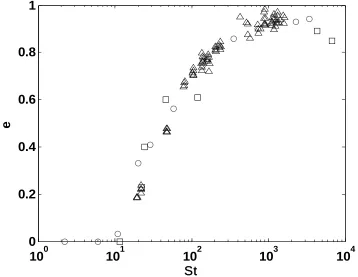
Figure 2.1. The effective coefficient of restitution as a function of the particle Stokes number for an immersed particle-on-wall normal collision in liquids. Steel and glass spheres collide on a stationary wall. (Ñ: McLaughlin 1968, ○: Gondret et al. 2002, and

Δ: Joseph et al. 2001)

When the sphere approaches the wall at high particle Stokes number, the viscous force becomes negligible, resulting in a nearly unity restitution coefficient, as if the collision took place in a dry medium. However, with decreasing particle Stokes number, the effective coefficient of restitution drops noticeably fromedry. When the particle Stokes

number falls below a critical value, a zero restitution coefficient is found, indicating no rebound motion, at least within the resolution of the image acquisition system.

The dependence of edry on particle Stokes number raises the question of whether a

(29)

12

upon impact. The mobility of the target particle necessitates the reexamination of the parameters: the effective coefficient of restitution and the particle Stokes number, which are used to characterize an immersed on-wall collision. In the current work, the experiments were conducted using spheres of identical size (D = 12.7 mm) but different

materials. Collisions between identical and dissimilar materials were examined. The experimental results are presented with the effective coefficient of restitution and a

binary Stokes number for a binary collision that will be defined in section 2.3.2. The

inter-particle collision result is also compared with the on-wall data.

2.2 Experiment setup

2.2.1 Apparatus

(30)

13

the liquid to settle down, ensuring a motionless target and a quiescent ambient fluid condition.

( a ) ( b )

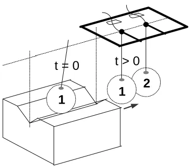
Figure 2.2. (a) Schematic experiment setup, side view, and (b) frontal sketch of the V-shaped release mechanism.

To control the inter-sphere distance upon impact, a precision fixture plate was designed, as shown in figure 2.3. Along the longitudinal plate centerline, two holes were drilled with a spacing of one sphere diameter and fine slots were cut to the side of the plate, allowing the passage of strings. The plate was aligned with the V-block guiding groove, ensuring an in-plane swinging motion. The tank was leveled and as a final calibration, one test collision was recorded from the frontal side to verify a head-on normal collision before each set of experiments.

t = 0 t > 0

1 1

2

(31)

14

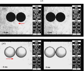
The sphere motion was recorded from the side or the bottom with a high-speed camera as described in Joseph (2003). The digital images were analyzed later to characterize the collision process. More details regarding the image processing can be found in section 2.2.3. In the cases with steel spheres, direct illumination resulted in bright areas on the mirror-like surface, as shown in figures 2.4(a) and 2.4(b). The uneven surface contrast caused problems in determining the sphere edge during the post-collision image analysis. In addition, the sphere blocked the light, blurring out the contact area, and made it difficult to locate the collision precisely in time. These problems were alleviated by new illumination method-background lighting. The tank was wrapped by translucent paper and illuminated from behind. The resulting images, as shown in figure 2.4(c), had sharper edges than those obtained with direct light. Also, the dark particles contrasted with the liquid well enough to determine the surface contour even upon contact. The method of background illumination also worked for semi-opaque glass spheres, as shown in figure 2.4(d).

- 5 ms 0 ms

( a )

- 4 ms 0 ms

(32)

15

0 ms - 5 ms

( c )

0 ms - 5 ms

( d )

Figure 2.4. Illumination effects. All the spheres are 12.7 mm in diameter. The camera position (side or bottom view), the sphere materials as impact-on-target, and the

illumination method are as follows: (a) Bottom view, steel-on-steel, direct illumination. (b) Bottom view, steel-on-Delrin, direct illumination. (c) Side view, steel-on-steel, background illumination. (d) Side view, glass-on-glass, background illumination.

2.2.2 Material properties

(a) Solid properties

Three types of 12.7 mm diameter solid spheres were used in the experiments: steel ball bearings, glass, and Delrin spheres. The spheres were identical to the ones used in Joseph (2003). The material properties and sphere surface roughness are summarized in Table 2.1, including solid density ρp, Young’s modulus E, Poisson’s ratioν, and the sphere

(33)

16

Table 2.1. Properties of the spheres used in collision experiments (Joseph 2003) Material _{(kg/m )}3

p

ρ (GPa)E ν σ_s(μm)

Steel 7780 190 0.27 0.0236 Glass 2540 60 0.23 0.134 Delrin 1400 2.8 0.35 0.796

(b) Liquid properties

The surrounding liquid was water-based glycerol solution whose viscosity varies significantly with temperature. Therefore, the liquid temperature was measure before each collision. The apparent specific weight of the solution was measured using a hydrometer for each set of experiments. The mixture density and viscosity can be extrapolated from the tables once the mixture composition is determined. The apparent specific weight of the liquids used in the current study ranged from 0% to 80%, which corresponds to a density ranging from 990–1210 _{kg m and a kinematic viscosity}3

of _{0.9 47 10 m s}₋ _× −6 2 _{. The solution properties with respect to apparent specific weight}

percentage are readily found (Joseph 2003).

2.2.3 Image analysis

(34)

17

grayness threshold in ImageJ1. During conversion, the RGB index of each pixel was transformed into a grayscale with unity and zero indicating true white and black, respectively. If one pixel has grayscale higher than the designated threshold, it is

converted into a white pixel; likewise a black pixel is created for pixels with grayscale lower than the threshold. The periphery of each sphere was determined by its peak contrast to the neighboring pixels with the outer radius representing the sphere surface. A black circle was obtained for steel and Delrin spheres, but a ring was generated for semi-opaque glass particles, as show in figure 2.5(b). The interior unity (white) pixels were replaced with zeros to represent the actual occupancy of the solid material in figure 2.5(c). The sphere centers were located at the mean X- and Y- coordinates of all the black pixels (zeros).

(a) (b)

(c)

Figure 2.5. Image conversion for a glass-on-glass collision (both 12.7 mm): (a) In RGB true color. (b) Black-and-white rings locating the spheres. (c) Filled binary image.

(35)

18

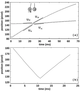
Each frame was converted and analyzed to determine the time evolution of the particle trajectories. A typical result is shown in figure 2.6(a); in figure 2.6(b), the estimated distance between sphere centers is plotted. The sphere trajectories were fitted in a least-squares sense (in MatLab) before and after the collision to calculate the impact and rebound velocities,Ui₁,Ur1,Ui2, andUr2. The resultant velocities slightly varied with

respect to the averaging duration. An average over 20 milliseconds would not capture the actual slowdown for a rapid collision. However, a time period shorter than 5 milliseconds does not reflect the real approaching velocity but pronounce only the decelerating particle motion. An intermediate time period, 10 to 15 milliseconds, was chosen such that the standard deviations for the four velocities are of the same order of magnitude in one collision.

0 5 10 15 20 25

120 130 140 150 160 170 180 gg2604-2 time (ms) di st anc e ( p ix el )

0 10 20 30 40 50 60 70 80 100 120 140 160 180 200 220 240 gg2604 time (ms) po si ti o n ( p ix el ) Ui1 U U U r1 r2 i2

( a )

( b ) 1 2

240 220 200 180 160 140 120 100 80 180 170 160 150 140 130 120

0 5 10 15 20 25

time (ms)

0 10 20 30 40 50 60 70

time (ms) p o s itio n (p ixel) pos it ion ( p ix e l)

Figure 2.6. Time evolution of (a) the particle trajectories and (b) the distance between the sphere centers. For this collision, the impact and rebound velocities areU_i₁ =65.6 mm s,

1 3.6 mm s

r

(36)

19

2.3 Physical

parameters

2.3.1 Coefficient of restitution in a liquid

Four velocities,Ui₁,Ui2,Ur1 andUr2, are involved in a particle-particle binary collision

rather than the two velocities, Ui andUr, for particle-wall collisions. Therefore a new

definition of the coefficient of restitution is required. Together with the particle Stokes number defined in equation (2.1), the coefficient of restitution, calculated by equation (2.3), successfully characterizes the particle-wall immersed collision. Therefore, it is reasonable to adopt the conventional definition:

1 2

r r

i i

U U

e

U U

− ≡ −

− , (2.4)

(37)

20

U _{i 1}

U _g

U r 1 U r 2

U _{i 2}

impact

compression

restitution

rebound time

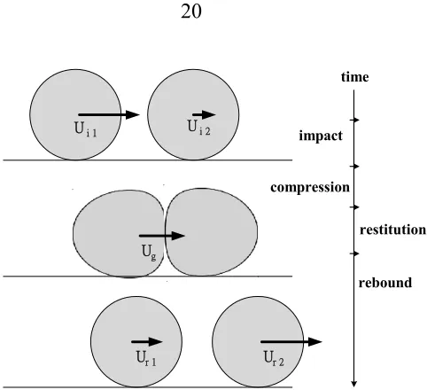
Figure 2.7. Schematic collision process.

As shown in figure 2.7, the impact sphere, of mass m₁, impacts the target sphere, of mass

and velocity m₂ andU_i₂, at a velocityU_i₁. During the compression phase, the contact

force rises and deforms both spheres and the two moves together at the group velocity:

1 1 2 2

0

1 2

i i

G

m U m U

U

m m

+ =

+ , (2.5)

which is derived from the conservation of linear momentum. The compression process affects the momentum of each sphere as:

1 1 1 0

2 2 2 0,

i c G

m U P m U

− =

⎧

⎨ ₊ ₌

⎩ (2.6)

where the compression impulse,

0 ( )

c

c c

P =

∫

τ F τ τd , is the time integration of the

compression force up to timeτc. The compression force F tc( )and durationτc can be

(38)

the first approximation, assuming a fully elastic deformation. However, without explicitly evaluating the integral, the contact impulse can be found by combining equations (2.5) and (2.6) to get:

1 2

( )

c i i

m m

P U U

m m

= −

+ .

Similar expressions for the restitution phase are readily found as:

1 0 1 1

2 0 2 2

G r r

m U P m U

− =

⎧

⎨ ₊ ₌

⎩ ,

involving three unknowns,

0 ( )

r

r r

P =

∫

τ F τ τd , U_r₁, and U_r₂, with only two equations.

Poisson’s hypothesis of P_r =e P_c can be used as the third equation to determine the

post-collision velocities as: 2

1 1 1 2

1 2

(1 ) ( )

r i i i

m

U U e U U

m m

= − + −

+ and

1

2 2 1 2

1 2

(1 ) ( )

r i i i

m

U U e U U

m m

= + + −

+ .

The coefficient of restitution is calculated as the ratio of restitution to compression impulse and can be expressed as the ratio of relative velocities before and after the collision:

1 2

r r r

c i i

P U U

e

P U U

−

= = −

− . (2.7)

(39)

22

2.3.2 Binary Stokes number

For a general binary immersed collision between objects of similar or dissimilar materials, sizes, and impact velocities, a binary Stokes number is proposed by considering the

hydrodynamic effects on the two approaching spheres. Following Poisson’s hypothesis, an immersed collision is also decomposed into a compression and a restitution phase. The momentum change of the impact sphere, including the hydrodynamic effects, is written as:

1 i1 c1 c 1 G

m U −H −P =m U , (2.8a)

with some intermediate group velocityU_G. The new term ₁ ₁

0 ( )

fc

c c

H =

∫

τ h τ τd estimates

the hydrodynamic impulse by integrating the total fluid force h t_c₁( ) up to timeτ_fc. The spheres make contact atτ_fc, initiating the physical compression process with a solid compression force. The compression force is integrated fromτ_fc toτ_fc+τ_c to determine the solid impulse P_c. After the general compression phase terminates at timeτ_fc+τ_c, the

general restitution phase commences and a momentum balance equation can be found for

the impact sphere as:

1 G r1 r 1 r1

m U −H −P =m U . (2.8b)

The sphere is decelerated by the fluid forceh tr₁( ), yielding the hydrodynamic rebound

impulse 2

1 ₀ 1( )

f

r r

H =

∫

τ h τ τd . A second set of equations can be derived for the target

(40)

23

2 i2 c2 c 2 g

m U −H +P =m U , (2.8c)

2 g r2 r 2 r2

m U −H +P =m U . (2.8d)

For both spheres, the solid impulses P_c and P_r are identical due to the mutual surface

contact. However, the hydrodynamic impulses are in general different, owing to the different particle sizes, solid densities, particle velocities, and ambient flows.

Using equations (2.8a)–(2.8d), the coefficient of restitution can be manipulated into:

1 2 1 2

*

1 1 2 2 1 2

1 2

1 2 1 2 1 2

*

1 1 2 2 1 2

r r r r r r r

g g

r r

i i c c c r r c c

g g

H P H P P H H

U U

m m m m m m m

U U

e

U U H P H P P H H

U U

m m m m m m m

⎛ ⎞ ⎛ ⎞ ⎛ ⎞ − − − − + + − ⎜ ⎟ ⎜ ⎟ ⎜ ⎟ − _⎝ _{⎠ ⎝} _⎠ _⎝ _⎠ = − = − = − ⎛ ⎞ ⎛ ⎞ ⎛ ⎞ + + − + − + − ⎜ ⎟ ⎜ ⎟ ⎜ ⎟ ⎝ ⎠ ⎝ ⎠ ⎝ ⎠ * 1 2 * 1 2 ( ) ( )

r r r H

c i i H

P m U U

+ Δ − Δ

=

+ Δ − Δ ,

where *

(

)

1

1 2

1 1

m = m + m − is defined as the reduced mass of the particle system. The

hydrodynamic effects are grouped into the parentheses subscripted “H.” For a dry binary

collision, there is no velocity change due to the fluid force, which corresponds to Poisson’s hypothesis for dry coefficient of restitution P_r =e P_c. For a particle-wall

immersed collision, where ΔU_r₂ = ΔU_i₂ =0 and m*=m_p, the coefficient of restitution,

* 1 1 * 1 1 ( ) ( )

r p r H

r r

i c p i H c

P m U

U P

e

U P m U P

+ Δ

= − = =

+ Δ ,

can be interpreted as the ratio of the generalized restitution and compression impulses, *

c

(41)

24

of the impact sphere due to the action of the hydrodynamic impulses. Therefore, for a sphere traveling at higher particle Stokes numbers, the momentum change (mpΔUi₁)H

will be smaller, resulting in a higher value of e. This correlation suggests a non-simple

dependence of the coefficient of restitution on St.

For a binary collision, the generalized impulses include the momentum change of the target sphere and the resulting expression is:

* *

1 2

* *

1 2

( )

r r r r H

c c i i H

P P m U U

e

P P m U U

+ Δ − Δ

= ≡

+ Δ − Δ .

Analogous to a particle-on-wall collision, the second term in the denominator represents the total momentum change in the particle system upon approaching and is assumed to be the controlling parameter for the total momentum loss during a collision. Following the correlation between(m_pΔU_i₁)_H and St, a binary particle Stokes number is proposed as:

*

*2

6

rel B

m U St

a

πμ

= . (2.9)

The particle system possesses reduced mass *

m and a reduced radius a* =

(

1a₁+1 a₂

)

−1,

while Urel =Ui₁−Ui₂ is the initial relative velocity between the two spheres. The

numerator of equation (2.9) provides a measure of available momentum in the solid phases that sustains the particle motion through the liquid and is identical to the original definition given in Davis, at al. (1986). Their definition was obtained upon solving the equation of motion for two approaching spheres whose motion is decelerated by the lubrication force.

(42)

25

viscous force, ₆ *

rel

a U

πμ , with a forcing duration *

rel

a U . For a particle-wall collision,

the time interval is a Ui and the original particle Stokes number, equation (2.1), is

recovered using * 1

m =m ,U_rel =U_i, and the viscous force 6πμaU_i. For a binary collision

between spheres of equal size, as used in the current experiments, the binary Stokes

number can be manipulated into:

*

2 Re 9

p

B rel

f

St ρ

ρ

= ,

with a reduced density *

(

)

1

1 2

1 1

p

ρ ρ ρ −

= + and a Reynolds number Re_rel =2aU_rel ν _f

based on relative velocity between the particles. Similarly, equation (2.1) can be written into St=

(

ρ ρp f

)

Re 9, which is widely used in the two-phase flow literature.

2.4 Normal

collisions

between

spheres of identical sizes

2.4.1 Identical spheres

The spheres used in the experiments were all 12.7 mm in diameter and were made of steel, glass, or Delrin. The effective coefficient of restitution for collisions between identical spheres is plotted versus the binary Stokes number in figure 2.8. A monotonic decrease ine with decreasing binary Stokes numbers is observed. A critical binary Stokes

number for zero coefficient of restitution, St_BC =2 ~ 8, was found, indicating either a fully stopped impact sphere before reaching the target or a zero relative velocity after collision. For some collisions in the most viscous liquid investigated in this study

( _{4.3 10 m s}5 2

f

(43)

26

restitution. The target sphere did not accumulate sufficient inertia to overcome the hydrodynamic forces and thus was unable to escape from the impact sphere. The critical binary Stokes number is lower than the value for particle-wall collisions (StC =7 ~ 12), which may result from the mobility for the target particle.

10

0

10

1

10

2

10

3

10

4

0

0.2

0.4

0.6

0.8

1 St

B

e

steel

glass

Delrin

Figure 2.8. Effective coefficient of restitution as a function of binary Stokes number for immersed normal collisions between identical spheres (D = 12.7 mm). The pair material

(44)

27

2.4.2 Dissimilar spheres

Within the same range of liquid viscosities, experiments involving collisions between spheres of identical size (12.7 mm) but dissimilar materials were also conducted. As shown in figure 2.9, a similar trend is observed of a monotonic decrease of coefficient of restitution with diminishing binary Stokes number.

10

0

10

1

10

2

10

3

10

4

0

0.2

0.4

0.6

0.8

1 St

B

e

s-g

g-s

s-D

g-D

(45)

28

In figure 2.10, the collision data for dissimilar spheres are compared with the results for identical pairs. The general agreement between the two data sets supports the use of the coefficient of restitution e= −(Ui₁−Ui₂) (Ur₁−Ur₂) and the binary Stokes number

* ₆ *2

B p rel

St =m U πμa to characterize the general binary immersed collision while a target

sphere, initially stationary, is free to move upon impact.

10

0

10

1

10

2

10

3

10

4

0

0.2

0.4

0.6

0.8

1 St

B

e

s-s

g-g

d-d

s-g

g-s

s-d

g-d

Figure 2.10. Immersed inter-particle normal collisions between identical and dissimilar spheres.

(46)

29

particles. The generalized compression impulse suggests a definition of the binary Stokes number for the pair and is shown to be well correlated with the coefficient of restitution.

2.4.3 Comparison with particle-wall collision

Furthermore, the inter-particle collision data are compared with the results of fully immersed collisions between a sphere and a stationary wall. As shown in figure 2.11, regardless of the target size and mobility, both dynamic collision process can be characterized by e and St_B, with the ambient fluid effects on the particle motion being

imbedded in StB. The effective coefficient of restitution for an immersed inter-particle

collision is slightly greater than the value for particle-wall collision, which can be attributed to the mobility of the target sphere. Moreover, boundary layers develop along the solid surfaces when the interstitial liquid is squeezed out upon the approach, a layer of which undergoes strong viscous dissipation consuming the momentum of the impact sphere. Such dissipation becomes weaker when the target is of finite size because of a smaller boundary layer. Thus a slightly greatere for particle-particle immersed collisions

is observed.

(47)

30

10

0

10

1

10

2

10

3

10

4

0

0.2

0.4

0.6

0.8

1 St

B

e

wall

s-s

g-g

d-d

s-g

g-s

s-d

g-d

Figure 2.11. Comparison of the inter-particle and the particle-wall immersed collisions.

(48)

31

around StB ≈50 130− , which is illustrated in figure 2.12. A linear-linear plot is used for this interested regime of StB. The interplay of the surface elements could also explain the

higher restitution for steel-on-glass collisions at around StB ≈10than for steel-on-steel impacts. However, the enhancement is less pronounced due to smaller particle inertia. For collisions at such low binary Stokes numbers, the hydrodynamic forces dominate the particle motion, diminishing the surface property effects on the rebound.

0

50

100

150

200

250

300

0

0.2

0.4

0.6

0.8

1 St

B

e

wall

s-s

g-g

d-d

s-g

g-s

s-d

g-d

(49)

32

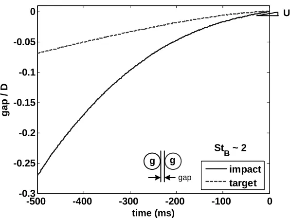
2.5 Particle motion with zero coefficient of restitution

In some immersed collisions, particularly those involving the most viscous liquid in the current experiments, the target sphere was observed to move, prior to contact, in the

same direction as the incoming sphere. The momentum of the impact sphere is transmitted to the target by the pressure front built up in the incompressible interstitial liquid layer.

(50)

33

-500 -400 -300 -200 -100 0

-0.3 -0.25 -0.2 -0.15 -0.1 -0.05 0

time [ms]

gap

/

D

gg 3700

impact target St

B ~ 2

g g

gap

UG

time (ms)

Figure 2.13. Time evolution of the interstitial gap for a glass-on-glass collision that results in zero restitution due to the nearly stopped impact sphere motion. Both glass spheres are 12.7 mm in diameter.

Unlike a particle-wall immersed collision where zero restitution results from either a fully stopped sphere upon contact or one that possesses insufficient rebound inertia for further reverse motion, an inter-particle collision can retain a post-collision group motion while a zero restitution coefficient is determined by equation (2.4). As depicted in figures 2.14(a) and 2.14(b), the target was accelerated from a non-zero velocity by the collision impulse. However, the impulse did not supply sufficient inertia for the target particle to overcome the hydrodynamic forces to separate further from the impact sphere. As a consequence, the two moved at a group velocity UG that is always lower than the dry group

velocity, 1 1 2 2 0

1 2

i i

G

m U m U

U

m m

+ =

+ from equation (2.5), due to the surrounding fluid effects. In

(51)

34

-20 -10 0 10 20 30 40

-0.15 -0.1 -0.05 0 0.05 0.1 0.15 0.2

time [ms]

ga

p /

D

sg 3672

B~7.5

s g

gap

U_G (a)

time (ms)

-20 0 20 40 60 80

-0.1 -0.05 0 0.05 0.1 0.15 0.2 0.25

time [ms]

gap

/ D

ss 3655

B ~11.2

s s

gap

U_G

(b)

time (ms)

(52)

35

If the group velocity in liquid,UG, is scaled by the dry group velocity,UG0, the group

efficiency number,

0

G G

G

U e

U

= ,

serves as an index of how efficient the pair particles move together under hydrodynamic forces. In figure 2.15, the binary Stokes number St_B is used to estimate the total fluid

force, as in the previous sections. When e_G is plotted against St_B, a decline in the group

efficiency number is observed when the binary Stokes number drops below 2, at which value the viscous force surpasses the solid inertia and severely dissipates the group motion. Since this type of group motion was rarely observed within the current impact conditions, further experiments would be needed for a quantitative description.

100 101

0 0.2 0.4 0.6 0.8 1

St

B

e G

s-s g-g s-g g-s

(53)

36

2.6 Summary

To summarize, Poisson’s impulse hypothesis that relates the compression and restitution process with the coefficient of restitution was used to estimate the total momentum loss during an immersed collision, between similar and dissimilar particles. The generalized compression impulse suggests a new definition of pertinent particle Stokes number for an inter-particle immersed collision-a binary Stokes number, StB. This number is shown to

be well correlated with the effective coefficient of restitution. While the effective coefficient of restitution, e , measures the resultant energy loss upon collision, the

ambient fluid effects are imbedded in the binary Stokes number. Despite the target size and mobility, the inter-particle collision data follow a similar trend to the results of particle-wall collisions. The general agreement supports the usage of e and St_B to

characterize such a rapid dynamic process.

(54)

37

Chapter 3 Wall Effects on the Hydrodynamic Forces

In chapter 2, a general correlation between the effective coefficient of restitution and the binary Stokes number was found for both inter-particle and particle-wall immersed collision. The monotonic decrease in the effective coefficient of restitution with diminishing binary Stokes number is expected to reveal the underlying physics of an immersed collision. A model that reproduces the correlation would be of particular use. The degree of collapse of the two data sets suggests the modeling of the sphere-wall collision as a first attempt to address how a second solid boundary affects the particle approaching motion. In order to describe the sphere motion in the proximity of wall, the conventional hydrodynamic forces, developed for the motion of a single sphere in an unbounded fluid domain, require modifications. The three forces examined in this chapter are: the steady viscous force, the added mass force, and the Basset history force.

3.1 Background

(55)

38

history force, which depends on the development of an unsteady boundary layer, was derived by Basset (1888) and Boussinesq (1885) independently for the force on a sphere that oscillates in the Stokes flow regime. Since then, extensive work has been done to extend these analytical expressions for a broader range of flow conditions. A thorough review can be found in Michaelides (1997).

The problem of the approach of a solid sphere towards a wall or another sphere in a viscous fluid forms an entire field of study. Brenner (1961) developed a correction term to Stokes’ drag for a rigid sphere with steady motion towards a wall at small Reynolds number. This value increases with diminishing gap width and converges to the classical lubrication theory when the gap drops to zero. Cox and Brenner (1967) applied a perturbation technique to extend this finding to sphere motion at higher Reynolds number where the liquid inertia becomes non-negligible. The new expression requires only a small gap Reynolds number, Re =g 2δ νU f , and can be used for particle motion beyond

(56)

39

3.2 Viscous

drag

3.2.1 Moderate Reynolds number effects

When the sphere is far away from wall, the viscous drag is calculated as:

6 ( )

D

F = − πμaUφ Re , (3.1)

where the correction on the Stokes’ drag,φ(Re), accounts for higher Reynolds number effects and is a function of the particle Reynolds number, Re = aU2 ν_f . It can be related to the steady state drag coefficient,C_D(Re), by:

( ) ( )

24

D

ReC Re

Re

φ = . (3.2)

Through out this work, the expression of ₍ _{) 1 0.15} 0.687

Re Re

φ = + is used for Re<800

(Clift, Grace, and Weber 1978). When the sphere moves close to the wall, the classical lubrication theory predicts a force that increases as the inverse of the gap width-a singular behavior not captured by equation (3.1).

3.2.2 Wall effects on the steady viscous drag

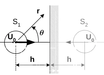
When the sphere moves closer to the wall, the small gap width ensures a Stokes’ flow between the solid surfaces. When the solid sphere moves at constant speed perpendicularly towards a wall atU , Brenner (1961) solved the quasi-steady Stokes’

(57)

*

6 ( )

D

F = − πμaUλ δ ,

where the non-dimensional gap, *

a

δ =δ , is scaled by the sphere radius a . The

correction factor, _{λ δ}_{( )}* _{, takes the form of an infinite series:}

( )

*

2 1 2 2

1 2

4 ( 1) 2sinh(2 1) (2 1)sinh 2

sinh 1

3 n (2 1)(2 3) 4sinh ( ) (2 1) sinh

n n n n

n n n n

α α

λ δ α

α α

∞ =

⎡ ⎤

+ + + +

= _⎢ − _⎥

− + _⎣ + − + _⎦

∑

, (3.3)

where_{α δ}_{( ) cosh (}* ₌ −1 _δ*₊₁₎_{. Cox and Brenner (1967) extended equation (3.3) for flow}

at higher Reynolds number, where the convective acceleration of the interstitial liquid becomes important and required only small gap Reynolds number Re=2δ νU _f . The

new wall correction term depends on both the gap width and the particle Reynolds number and is given by:

* 1 *

4

* *

1 1 1

( , ) 1 (1 ) log 5

Re Re

λ δ δ

δ δ

⎡ ⎤

≈ _⎢ + ± _⎥

⎣ ⎦. (3.4)

Cox and Brenner’s sign convention is adopted. For an approaching sphere, a plus sign in front of the particle Reynolds number is used and it is switched to a negative when the sphere rebounds from the wall. The wall-modified viscous drag can thus be written as:

*

6 ( , )

D

F = − π μa U λ δ Re . (3.5)

Interaction law for a collision between two solid particles in a viscous liquid