Determination Of Adaptive Control Parameter Using Fuzzy Logic Controller

(1)

243

Determination Of Adaptive Control Parameter

Using Fuzzy Logic Controller

Omur Can Ozguney, Recep Burkan

Abstract: The robot industry has developed along with the increasing the use of robots in industry. This has led to increase the studies on robots. The

most important part of these studies is that the robots must be work with minimum tracking trajectory error. But it is not easy for robots to track the desired trajectory because of the external disturbances and parametric uncertainty. Therefore, adaptive and robust controllers are used to decrease tracking error. The aim of this study is to increase the tracking performance of the robot and minimize the trajectory tracking error. For this purpose, adaptive control law for robot manipulator is identified and fuzzy logic controller is applied to find the accurate values for adaptive control parameter. Based on the Lyapunov theory, stability of the uncertain system is guaranteed. In this study, robot parameters are assumed to be unknown. This controller is applied to a robot model and the results of simulations are given. Controller with fuzzy logic and without fuzzy logic are compared with each other. Simulation results show that the fuzzy logic controller has improved the results.

Keywords: Fuzzy Logic Control, Lyapunov Stability, Adaptive Control, Robotics.

————————————————————

1 Introduction

Spong [1], derived a simple adaptive nonlinear control law for n-link robot manipulators. Passivity-based approach is used and the stability of the uncertain system is guaranteed based on the Lyapunov theory. This methodology has some advantages about both robustness and design. Er and Gao [2] designed a robust adaptive fuzzy neural controller for multilink manipulators. Asymptotic stability of the control system is established using the Lyapunov theory. This study shows that tracking errors and handled external disturbances are compensated by this new controller. Tayebi [3] represents adaptive iterative learning control for rigid robot manipulators. This model includes unknown parameters. This control was designed based on a proportional-derrivative feedback control. The simulation results show the effectiveness of the proposed controller. An integration of kinematic controller and a torque controller was presented by Fukao, Nakagawa and Adachi [4]. First a new adaptive control law was introduced than a torque adaptive controller derived by using this new adaptive kinematic controller. The controller was applied to a nonholonomic mobile robot. The results show that for proposed controller was effective at values of angular velocity approaching zero. Fateh and Farhangfard [5] discussed the uncertainties of the Jacobian matrix in the control system. The trajectory tracking error in the task space was improved by using the new controller. Feedback linearization is the main part of this control method. Massoud, Elmaraghy and Lahdhiri [6] used a feedback linearization, a sliding mode technique, and a LQE methodology together. The controller takes advantages of these control methods and the new control method was applied to flexible joint manipulator. The results showed that the developed controller was successful in end-point position control.

Fateh [7] improves his previous study [8] and applied to a three-joint articulated ﬂexible-joint robot. This study based on torque control strategy. Stability of the system was guaranteed and performance of the control system is evaluated. In this paper, a new fuzzy-adaptive control law is developed based on the Lyapunov function, thus stability of the system is guaranteed. First, adaptive control law is identified then, control parameter is defined by fuzzy logic controller. After simulation results, it has been seen that fuzzy logic controller improve the performance of the adaptive control law.

2 STABILITY ANALYSIS AND DEFINITION OF

THE ADAPTIVE CONTROL LAW

In the absence of friction or other disturbances, the dynamic model of an n-link manipulator can be written as[1];

M ( q ) qC ( q , q ) qG ( q )τ (1)

where q denotes generalized coordinates, τ is the n-dimensional vector of applied torques (or forces), M(q) is the nxn symmetric positive definite inertia matrix, ̇ ̈ is the n-dimensional vector of centripetal and Coriolis terms and G(q) is the n-dimensional vector of gravitational terms.

With n

qR , R which has both the skew-symmetry property that the matrix [9];

N ( q , q ) = M ( q ) - 2 C ( q , q ) (2)

is skew-symmetric. Equation (1) can be also written in the following form.

M ( q ) qC ( q , q ) qG ( q )Y ( q , q , q )   (3)

Where  is a constant p-dimensional vector of robot parameters and Y is an nxp matrix of known functions of joint position, velocity and acceleration. We can say that is

uncertain if there exists 0 R , R 



    both known, such that

[1]

0

       (4)

_________________________

 Omur Can Ozguney is currently pursuing phd program in mechanical engineering in Istanbul University, Turkey, E-mail: omur.ozguney@istanbul.edu.tr

(2)

As distinct to similar study [10],  and are unknown. The

nominal control vector ₀ is described as [1];

0 0 0 0 D

r r 0 D

τ M ( q ) a C ( q , q ) v G ( q ) K r

Y ( q , q , q , q ) K r

   

  

(5)

The quantities v, a and r is defined as;

d d

vq  q ; av ; r  q q ; q q q (6)

Where KD and  are positive definite matrix and q d

is reference trajectory. The control input is defined in terms of the nominal control vector ₀as [1];

0

0 D

τ τ + Y ( q , q , v , a ) u

= Y ( q , q , v , a ) ( u ) K r



  

(7)

Where u is an additional control input. Substituting eq. (7) into eq. (1) it can be define;

D

M ( q ) rC ( q , q ) rK rY ( q , q , v , a ) ( u ) (8)

Based on these definitions, the following theorem is given.

Theorem 1: [1]

T

T T

2

T T

Y r

ˆ _{i f} ˆ _Y _r

Y r

u ˆ

ˆ Y r i f Y r



    

   

 

 _ _{ }

 _ 

(9)

and choose ˆ and according to;

T

ˆ _L _Y _r

l

 

   

(10)

The control law (7) is continuous and the closed loop system is globally convergent, i.e., the position and velocity tracking errors, ̃, and ̃̇, respectively, converge asymptotically to zero while all signals remains bounded.

Proof [1]:

The stability of the system is guaranteed by using the Lyapunov function. The following part of this study is given in [1].

3 FUZZY LOGIC CONTROLLER

There are several studies related with fuzzy logic controller.[11],[12],[13],[14]. There are several vague linguistic expressions (small, medium,large) can be expressed as by membership functions. These membership functions are triangular, trapezoidal or bell curved shape. (Fig. 1). They take the values between [0,1].

Fig. 1.Different shapes of membership functions [15]

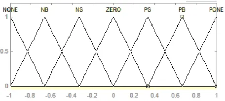
There are three steps of the fuzzy logic control. In the Fuzzification stage, membership functions are defined for the variables. Thus, certain values are converted to fuzzy values. The second stage is the rule evaluation step. The rules have been prepared based on the knowledge of the system. And the output of the system is decided by the input of the system. And the final part is the defuzzification step. In this part, fuzzy values converted to certain values. Fuzzy Logic Controller has three inputs and one output. These are errors of joints (e1,e2,e3), and control parameter (L) respectively. Linguistic variables which implies inputs and output have been classified as: NONE, NB, NS, Z, PS, PB, PONE. Inputs and output are all normalized in the interval of [0, 1] as shown in Fig.2

Fig. 2. Membership functions of inputs (e1,e2,e3) and

output (L)

The linguistic labels used to describe the Fuzzy sets were ―Negative One‖ (NONE), ―Negative Big‖ (NB), ―Negative Small‖ (NS), ―Zero‖ (Z), ―Positive Small‖ (PS), ―Positive Big‖ (PB), ―Positive One‖ (PONE). The fuzzy control rule is in the form of:IF e=Ei and de=dEj THEN L = L(i,j), These rules are written in a rule base look-up table which is shown in Table 1

TABLE 1

DECISION TABLE (L)

e1\e2\

e3 NONE NB NS Z PS PB

PON E NON

E NONE NONE NB NB

N

S NS Z

NB NONE NB NB NS N

S Z PS

NS NB NB NS NS Z PS PS

Z NB NS NS Z PS PS PB

PS NS NS Z PS PS PB PB

PB NS Z PS PS PB PB PON

E

PONE Z PS PS PB PB PON

E

PON E

4 DYNAMIC

EQUATIONS

OF

THE

THREE

AXIS

ROBOT

ARM

(3)

245

Fig. 3. Three axis robot arm [16]

Where m1 and m2 are masses of the links, L1 and L2 are the

lengths of the links, I1, I2 and I3 are the mass inertia of the

links and q1, q2 and q3 are the angles of the links. Also the

torques are represented in a matrix form like in (11) [17]

1 1 1 2 1 3 1

2 1 2 2 2 3 2

3 1 3 2 3 3 3

1 1 1 2 1 3 1 1 1 1

2 1 2 2 2 3 2 2 1 2

3 1 3 2 3 3 3 3 1 3

M M M q

C C C q G q

          _ _{ } _                         _ _{ } __ _{ } _                 (11) 2 2 1

1 1 1 1 2 2

2 2

2 1 2 2 3 2 3 2 2 3 1 2 l

M I ( m ( ) I ) c o s q

2

l

m l [ l c o s q l c o s q c o s q ] ( m ( ) I ) c o s q 2

  

   

1 2 1 3 2 1 3 1

M 0 , M 0 , M 0 , M 0

2 2 2

1 2

2 2 1 2 21 21 2 3 2 3

l l

M ( m ( ) I ) m l m l l c o s q ( m ( ) I )

2 2

     

2 2

2 3 2 1 3 2 3

l l

M m l ( ) c o s q m ( ) I

2 2

  

2 2

3 2 2 1 3 2 3

l l

M m l ( ) c o s q m ( ) I

2 2

   ,

2 2

3 3 2 3

l

M m ( ) I

2

 

2 2

1 1 2 3 2 3 2 3 2 3 l

C 2 ( ( m ( ) I ) s i n q c o s q ( q q ) ) 2

  

2 1

1 2 2 2

1 2 1

2 2 2

21 2 2 2 1 2 2 3

l

( m ( ) I ) s i n q c o s q

2

C 2 q

l

m l s i n q c o s q m l ( ) s i n q c o s q

2         _ _ _ _      2 2

1 3 2 1 2 2 3 1

l

C ( 2 m l ( ) c o s q s i n q ) q 2



2 2

1

1 2 2 2 2 1 2 2

2 1 1

2 2

2 1 2 2 3 2 3 2 3 2 3

l

( m ( ) I ) s i n q c o s q m l s i n q c o s q

2

C q

l l

m l ( ) s i n q c o s q ( m ( ) I ) s i n q c o s q

2 2               _ _      2 2

2 2 2 1 3 3

l

C ( 2 m l ( ) s i n q ) q 2



2 2

2 3 2 1 3 3

l

C ( m l ( ) s i n q ) q

2



2 2

2 1 2

3 1 2 3 1

2 2

2 3 2 3

l

( m l ( ) s i n q )

2

C c o s q q

l

( m ( ) I ) s i n q

2           _ _      2 2

3 2 2 1 3 2 l

C ( m l ( ) s i n q ) q

2

 

3 3

C  0

1 1

G  0

1 2

2 1 1 2 2 1 2 2 2 3

l l

G g m c o s q g m l c o s q g m c o s q

2 2

  

2

3 1 2 2 3

l

G g m c o s q

2

 (12)

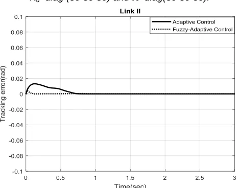
The simulations have been done under the maximum uncertainty (worse case) using the control law (9). In order to investigate the performance of the new and previous controller [1], each control law with the same control parameters such as Kd= diag(30 30 30) and =diag(30 30

30) is applied to the same model system using same trajectory. The obtained results for Kd and  are plotted in

Figures 4-9.

Fig. 4. Response using the adaptive control law (9) and

fuzzy-adaptive control law with (0.1*cos(t)) trajectorywhen Kd=diag (30 30 30) =diag (30 30 30).

Fig. 5. Response using the adaptive control law (9) and

(4)

Fig. 6. Response using the adaptive control law (9) and fuzzy- adaptive control law with (0.1*cos(t)) trajectory when

Kd=diag (30 30 30) =diag(30 30 30),

Fig. 7. Response using the adaptive control law (9) and

fuzzy-adaptive control law with (0.5*sin(t))) trajectory when Kd=diag (30 30 30) and =diag(30 30 30).

fuzzy-adaptive control law with (0.5*sin(t))) trajectory when Kd=diag(30 30 30) and =diag(30 30 30).

As seen from Figures 4-9, tracking performance of the system changes depending on the values of the control gain L. Tracking performance of the fuzzy-adaptive is better then the adaptive control law (9). Tracking performance of the controller is improved by the fuzzy logic control parameter of L.

5 C

ONCLUSION

The aim of this study is to develop a novel fuzzy-adaptive control law in order to increase tracking performance of the robot manipulators. For this purpose, a fuzzy logic control rule is designed for control parameter L. In the previous study [1], the control gain is constant. The novelty of this project is that the control gain is defined by fuzzy logic controllers. As shown from Fig. 4-11, tracking performance of the proposed fuzzy-adaptive control law is better than the developed adaptive control law (9). Tracking performance of the controller changes depending on the values of the control gain L, and tracking performance can be improved by using fuzzy logic controller for the control gain to appropriate values. As seen from Fig. 4-11, the proposed fuzzy-adaptive control law increases tracking performance of the system.

References

[1]. Spong, M. W., ―Adaptive control of robot manıpulators design and robustness‖, American Control Conference, 2-4 June 1993 Urbana, pp. 2826-2830.

[2]. Er, M. J. and Gao M., ―Robust adaptive control of robot manipulators using generalized fuzzy neural networks‖, IEEE Transactions on Industrial Electronics, V. 50, N. 3, June 2003, pp. 620-628.

[3]. Tayebi, A., ―Adaptive iterative learningcontrol for robot manipulators‖, Automatica, 40, 2004, pp.1195-1203.

(5)

247

IEEE Transactions on Robotıcs and Automation, V. 16, N. 5, October 2000, pp. 609-615.

[5]. Fateh, M. M. and Farhangfard, H., ―Reducing the error of manipulator jacobian in the control system‖, Proceedings of the 2nd WSEAS International Conference on Dynamical Systems and Control, Bucharest, Romania, 2006, pp.13-17.

[6]. Massoud, A. T., Elmaraghy, H. A., and Lahdhırı, T., ―On the Robust Nonlinear Motion Position and

Force Control of Flexible Joints Robot

Manipulators‖, Journal of Intelligent and Robotic Systems, Netherlands,25, 1999, pp.227–254.

[7]. Fateh, M. M., ―Robust control of flexible-joint robots using voltage control Strategy‖, Nonlinear Dyn., 67, 2012, pp.1525–1537.

[8]. Fateh, M. M.. ―Robust voltage control of electrical manipulators in task-space‖ Int. J. Innov. Comput. Inf. Control 6(6), 2010, 2691–2700.

[9]. Spong, M.W., and Vidyasagar, M., Robot

Dynamics and Control, John Wiley & Sons, Inc., New York, 1989.

[10]. Silotine, J-J. And Li, W., "On the Adaptive Control of Robot Manipulators," Lot. J: Robottics Research, Vol. 6, No. 3, 1987. pp. 49-59.

[11]. Yoshimura, T.,Isari, Y, LI, Q., and Hino J., ―Active Suspension of Motor Coaches Using Skyhook Damper and Fuzzy Logic Control, Control Eng. Practice, Vol. 5, No. 2, 1997 pp. 175-184.

[12]. Yoshimura, T., Nakaminami, K., Kurimoto, M., and Hino, J., ―Active suspension of passenger cars using linear and fuzzy-logic controls‖, Control Engineering Practice 7 1999, pp.41-47.

[13]. Shukla, S., and Tiwari, M., ―Fuzzy Logic of Speed

and Steering Control System for Three

Dimensional Line Following of an Autonomous Vehicle‖, (IJCSIS) International Journal of Computer Science and Information Security, Vol. 7, No. 3, 2010, pp. 101-108.

[14]. Turkkan, M., and Yagiz, N., ―Fuzzy logic control for active bus suspension system‖, International Conference on Mathematical Modelling in Physical Sciences, Journal of Physics: Conference Series 410, 2012, pp.1-4.

[15]. Hacioglu, Y., ―Bir Robotun Bulanık Mantıklı Kayan Kipli Kontrolü‖, Yüksek Lisans Tezi, İstanbul Üniversitesi Fen Bilimleri Enstitüsü, 2004.

[16]. Ozguney, O., ―Model Parametreleri Bilinmeyen Mekanik Manipulatörlerin Kontrolü‖, Yüksek Lisans Tezi, İstanbul Üniversitesi Fen Bilimleri Enstitüsü, 2012.

[17]. Rivin, E.I., ―Mechanical Design of Robots‖, McGraw-Hill, New York,1987.

Appendix A

Table 2

Parameters of the unloaded arm

m1 m2 l1 l2 lc1 lc2 I0 I1 I2