Decision Making
Research article
A comparative analysis of multi-level computer-assisted decision
making systems for traumatic injuries
Soo-Yeon Ji*
1, Rebecca Smith
1, Toan Huynh
2and Kayvan Najarian
1Address:1Department of Computer Science, Virginia Commonwealth University, 401 East Main Street, Richmond, Virginia, USA and 2Department of Surgery, Carolinas Healthcare System, Charlotte, NC, USA
E-mail: Soo-Yeon Ji* - [email protected]; Rebecca Smith - [email protected]; Toan Huynh - [email protected]; Kayvan Najarian - [email protected];
*Corresponding author
Published: 14 January 2009 Received: 1 February 2008
BMC Medical Informatics and Decision Making2009,9:2 doi: 10.1186/1472-6947-9-2 Accepted: 14 January 2009 This article is available from: http://www.biomedcentral.com/1472-6947/9/2
©2009 Ji et al; licensee BioMed Central Ltd.
This is an Open Access article distributed under the terms of the Creative Commons Attribution License (http://creativecommons.org/licenses/by/2.0), which permits unrestricted use, distribution, and reproduction in any medium, provided the original work is properly cited.
Abstract
Background: This paper focuses on the creation of a predictive computer-assisted decision making system for traumatic injury using machine learning algorithms. Trauma experts must make several difficult decisions based on a large number of patient attributes, usually in a short period of time. The aim is to compare the existing machine learning methods available for medical informatics, and develop reliable, rule-based computer-assisted decision-making systems that provide recommendations for the course of treatment for new patients, based on previously seen cases in trauma databases. Datasets of traumatic brain injury (TBI) patients are used to train and test the decision making algorithm. The work is also applicable to patients with traumatic pelvic injuries.
Methods: Decision-making rules are created by processing patterns discovered in the datasets, using machine learning techniques. More specifically, CART and C4.5 are used, as they provide grammatical expressions of knowledge extracted by applying logical operations to the available features. The resulting rule sets are tested against other machine learning methods, including AdaBoost and SVM. The rule creation algorithm is applied to multiple datasets, both with and without prior filtering to discover significant variables. This filtering is performed via logistic regression prior to the rule discovery process.
Results: For survival prediction using all variables, CART outperformed the other machine learning methods. When using only significant variables, neural networks performed best. A reliable rule-base was generated using combined C4.5/CART. The average predictive rule performance was 82% when using all variables, and approximately 84% when using significant variables only. The average performance of the combined C4.5 and CART system using significant variables was 89.7% in predicting the exact outcome (home or rehabilitation), and 93.1% in predicting the ICU length of stay for airlifted TBI patients.
Conclusion: This study creates an efficient computer-aided rule-based system that can be employed in decision making in TBI cases. The rule-bases apply methods that combine CART and C4.5 with logistic regression to improve rule performance and quality. For final outcome prediction for TBI cases, the resulting rule-bases outperform systems that utilize all available variables.
Background
According to a 2001 National Vital Statistics Report [1], nearly 115,200 deaths occur each year due to traumatic injury, and many patients who survive suffer life-long disabilities. Among all causes of death and permanent disability, traumatic brain injury (TBI) is the most prevalent. Of the 29,000 children who are hospitalized each year with TBI, a significant percentage will suffer from neurological impairment [2]. It has also been reported that the traumatic brain injuries are the most expensive affliction in the United States, with an estimated cost of $224 billion [3].
Computer-aided systems can significantly improve trauma decision making and resource allocation. Since trauma injuries have specific causes, all with established methods of treatment, fatal complications and long-term disabilities can be reduced by making less subjective and more accurate decisions in trauma units [4]. In addition, it has been suggested that an inclusive trauma system with an emphasis on computer-aided resource utiliza-tion and decision making may significantly reduce the cost of trauma care [1].
Since the treatment of traumatic brain injuries is extremely time-sensitive, optimal and prompt decisions during the course of treatment can increase the likelihood of patient survival [5, 6]. It is also believed that the predicted length of stay in the ICU is an important factor when deciding on the patient transport method (i.e. ambulance or helicop-ter), as more critical patients are expected to spend more time in the ICU, and these stand to benefit the most from helicopter transport. Studies have emphasized the critical impact of helicopter transport on trauma mortality rates, since the speed of ambulance transport is limited by road and weather conditions, and may also be constrained by traffic congestion. However, it is difficult to compare ground and helicopter transportation and the correspond-ing care provided to the patients [7]. Cunncorrespond-ingham [8] attempts a comparison based on the outcome of the treatment given to trauma patients. Based on his study, patients in critical condition are more likely to survive if transported via helicopter. However, the high cost of helicopter transport remains a major problem [9, 10]. In recent studies, Gearhart evaluated the cost-effectiveness of helicopter for trauma patients and suggested that on average the helicopter transport cost is about $2,214 per patient, and $15,883 for each additional survivor [11]. Eventually, the cost is almost $61,000 per surviving trauma patient. Eckstein [12] states that 33% of patients who are transported by helicopter are discharged home from the emergency department [12], rather than being sent to ICU. This indicates that a significant number of trauma patients transported by helicopter actually have relatively minor
injuries. This emphasizes the necessity of a comprehensive transport policy based on patient condition and predicted outcome.
Several computer-assisted systems already exist for decision-making in trauma medicine. The majority of these systems [13, 14] are designed to perform a statistical survey of similar cases in trauma databases, based only on patient demographics. As such, they may not be sufficiently accurate and/or specific for practical implementation. Other medical decision making sys-tems employ the predictive capabilities of artificial neural networks [15-17]; however, due to the 'black box' nature of these systems, the reasoning behind the predictions and recommended decisions is obscured. Currently, none of these existing systems are in wide-spread use in trauma centers. There are three main reasons: the use of non-transparent methods, such as neural networks; the lack of a comprehensive database integrating all relevant available patient information for specific prediction processes; and poor performance due to the exclusion of relevant attributes and the inclusion of those irrelevant to the current task, resulting in rules that are too complicated to be clinically meaningful.
Therefore, a possible approach to create accurate and reliable rules for decision making is to combine machine learning and statistical techniques [23, 24]. This paper analyzes the performance of several combinations of machine learning algorithms and logistic regression, specifically in the extrac-tion of significant variables and the generaextrac-tion of reliable predictions. Though a transparent rule-based system is preferable, other methods (such as neural networks) are also tested in the interest of comparision. A computational model is developed to predict final outcome (home or rehab and alive or dead) and ICU length of stay. In addition, we identify the factors and attributes that most affect decision making in the treatment of traumatic injury.
Our hypotheses are as follows:
1. We hypothesize that a rule-based system, attractive to physicians as the reasoning behind the rules is transpar-ent and easy to understand, can be as accurate as "black-box" methods such as neural networks and SVM.
2. We hypothesize that when trained correctly, a computer-aided decision making system can provide clinically useful rules with a high degree of accuracy.
3. Studies mentioned earlier have examined which variables are most significant in the recommendation/ prediction making process. We hypothesize that airway status, age, and pre-existing conditions such as myocardial infarction and coagulopathy are significant variables.
Methods
Rules are created by processing patterns discovered in the traumatic brain injury (TBI) datasets. More specifically, they are generated by analyzing the logical and gram-matical relationships among the input features and the resulting outcomes. Rules are formally defined as grammatical expressions of knowledge extracted using specific logical operations on the available features [6].
CART and C4.5 are among the most popular algorithms for creating reliable rules, but they are limited in their ability to identify the most significant variables. We therefore perform statistical analysis using logistic regression, which is typically effective in discovering statistically significant regression coefficients [24]. Although stepwise regression is designed to find significant variables, it may not perform well with CART when dealing with small scale datasets [25]. There-fore, in this paper, logistic regression with direct maximum likelihood estimation (Direct MLE) is used.
Dataset
Three different datasets are used in the study: on-site, off-site, and helicopter. The on-site dataset contains data
captured at the site of the accident; the off-site dataset is formed at the hospital after patients are admitted; and the helicopter dataset consists of the records for patients who are transported to hospital by helicopter. The on and off-site datasets are used to predict patient survival (dead/alive) and final outcome (home/rehab), and the helicopter dataset is used to predict ICU length of stay, which is a measure used in estimating the need for helicopter transportation. The datasets are provided to us by the Carolinas Healthcare System (CHS) and the National Trauma Data Bank (NTDB).
On-site dataset
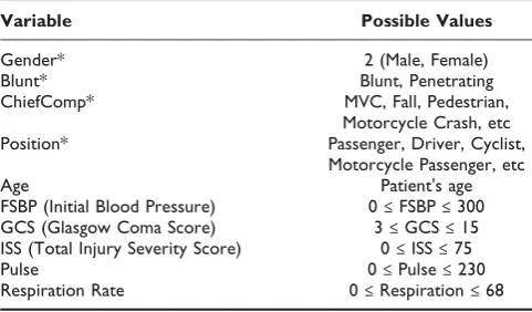
When making decisions based on the variables available at the accident scene, one has to consider the unavail-ability of important factors such as pre-existing condi-tions (comorbidities). Decisions must therefore be made without knowledge of these factors. Some physiological measurements are also excluded because they are only collected after arrival at the hospital. Table 1 presents the variables collected for this dataset, which consist of four categorical and six numerical attributes.
Off-site dataset
The off-site dataset contains information on comorbid-ities and complications, and includes all variables. A total of 1589 cases are included in the database: 588 fatal and 1001 non-fatal. The inputs include both categorical and numerical attributes. The predicted outcomes are defined as the patients' survival, i.e. alive or dead, and the exact outcome for surviving patients, i.e. rehab or home.
Table 2 presents the variables for our dataset. Among the categorical variables, "prexcomor" represents any comor-bidities that may negatively impact a patient's ability to recover from the injury and any complications. Other terms are defined in the table description.
Table 1: On-site dataset
Variable Possible Values
Gender* 2 (Male, Female)
Blunt* Blunt, Penetrating
ChiefComp* MVC, Fall, Pedestrian,
Motorcycle Crash, etc
Position* Passenger, Driver, Cyclist,
Motorcycle Passenger, etc
Age Patient's age
FSBP (Initial Blood Pressure) 0≤FSBP≤300
GCS (Glasgow Coma Score) 3≤GCS≤15
ISS (Total Injury Severity Score) 0≤ISS≤75
Pulse 0≤Pulse≤230
Respiration Rate 0≤Respiration≤68
Helicopter dataset
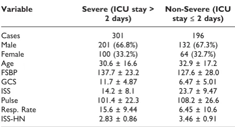
This dataset is formed based on the records of patients who were transported to hospital by helicopter. The variables are age, gender, blood pressure, cheifcomp (the type of injury), airway (the type of device used to assist patients with breathing), prefluids (the amount of blood provided to the patients), GCS, heart rate, respiration rate, ISS-Head&Neck, and ISS. Age, blood pressure, GCS, heart rate, ISS-Head&Neck, ISS, and respiration rate are classified as numerical variables. The final outcome is the number of days spent in ICU, as this is considered the most informative measure when deciding the means of transport to hospital. In our dataset, ICU stay ranges between 0 and 49 days. The use of a relatively small dataset with so many outcomes may result in a complex model that is hard to explain and understand. Inspired by Pfahringer [26], the dataset is classified into two groups. The non-severe group contains patients who stayed in the ICU less than 2 days (ICU stay≤2 days). The severe group consists of patients who stayed in the ICU more than 2 days (ICU stay ≥ 3 days). This threshold was chosen based on discussion with trauma experts. In total, the dataset contains 497 cases: 196 severe and 301 non-severe [10]. Table 3 describes the helicopter dataset in more detail.
Learning algorithms
It is known that the patterns observed in trauma cases are often extremely complicated; that is, the treatment
outcomes for two apparently similar patients may turn out to be significantly different. Linear methods have proven insufficient even in the analysis of patterns as simple as the "exclusive-or" function. Because these limitations are inherited by linear regression methods, the use of non-linear techniques for computer-aided trauma systems has been broadly encouraged [27]. Neural networks are a common choice; however, they are not transparent, since the knowledge learned from the training examples is hidden within the structure and weights of the networks [28]. While there are existing Table 2: Off-site dataset
Variable Alive Dead Rehab Home
Cases 1001 588 628 213
Male* 704 (70.3%) 404 (68.7%) 443 (70.5%) 150 (70.4%)
Female* 297 (29.7%) 184 (31.3%) 185 (29.5%) 63 (29.6%)
Age 41.2 ± 19.6 49.2 ± 24.1 39.6 ± 19.3 37.2 ± 16.6
FSBP 126 ± 33.4 119.3 ± 45.6 125.3 ± 31.6 124.5 ± 34.1
FURR 15.3 ± 10.9 13.9 ± 11.9 14.4 ± 11.1 18.2 ± 10.5
GCS 8.7 ± 5.3 27.5 ± 5.2 7.9 ± 5.2 10.5 ± 5.1
ISS 30.5 ± 12.8 35.3 ± 14.7 32 ± 13.2 27.1 ± 11.7
EDEYE 2.4 ± 1.4 2.1 ± 1.4 2.2 ± 1.4 2.8 ± 1.4
ED Verbal 2.7 ± 1.8 2.3 ± 1.7 2.4 ± 1.8 3.3 ± 1.8
EDRT 4.6 ± 3.2 3.8 ± 3.3 4.1 ± 3.3 5.7 ± 2.89
Head AIS 3.0 ± 1.6 3.6 ± 1.6 3.1 ± 1.8 2.5 ± 1.4
Thorax AIS 2.3 ± 1.7 2.4 ± 1.8 2.3 ± 1.8 2.4 ± 1.7
Abdomen AIS 1.1 ± 1.5 1.1 ± 1.6 1.0 ± 1.5 1.5 ± 1.7
Intubation* Yes/No
Prexcomor* 17 values: Acquired Coagulopathy, Chronic Alcohol Abuse, Chronic Obstructive Pulmonary Disease, Congestive
Heart Failure, Coronary Artery Disease, Coumadin Therapy, Documented History of Cirrhosis, Gastric or Esophageal Varices, Hypertension, Insulin Dependent, Myocardial Infarction, Non-Insulin Dependent, Obesity, Pre-existing Anemia, Routine Steroid Use, Serum Creatinine > 2 mg % (on Admission), Spinal Cord Injury
Complications* Acute Respiratory Distress Syndrome (ARDS), Aspiration Pneumonia, Bacteremia, Coagulopathy, Intra-Abdominal
Abscess, Pneumonia, Pulmonary Embolus
Safety* Seat Belt, None Used, Air Bag Deployed, Helmet, Other, Infant/Child Car Seat, Protective Clothing
First, the number of cases in each group (Alive, Dead–and within the surviving patients, Rehab and Home) is listed. For the numerical attributes, the table provides Mean ± Standard Deviation. Finally, the categorical variables are listed with all their possible values. ISS provides the overall injury severity score (ISS) for patients with multiple injuries, and GCS is the Glasgow Coma Score. Many studies make heavy use of GCS and ISS, as these measures are considered standard metrics in assessing patient condition and degree of injury. Note that surviving patients who were transported to other hospitals are not included in the rehab + home total.
Table 3: Helicopter dataset
Variable Severe (ICU stay > 2 days)
Non-Severe (ICU stay≤2 days)
Cases 301 196
Male 201 (66.8%) 132 (67.3%)
Female 100 (33.2%) 64 (32.7%)
Age 30.6 ± 16.6 32.9 ± 17.2
FSBP 137.7 ± 23.2 127.6 ± 28.0
GCS 11.7 ± 4.87 6.47 ± 5.01
ISS 14.2 ± 8.1 23.7 ± 9.47
Pulse 101.4 ± 22.3 108.2 ± 26.6
Resp. Rate 15.6 ± 9.44 6.45 ± 10.6
ISS-HN 2.83 ± 0.86 3.46 ± 0.91
methods that can extract approximate rules to represent this hidden knowledge, they cannot truly represent the trained networks [6]. Support Vector Machines (SVM's) and AdaBoost share the same problem: the knowledge used in the decision making process is not visible to humans, a requirement that is extremely important in medical applications. Rule-based methods such as CART and C4.5 provide completely transparent computational decision making systems while still utilizing some nonlinear capabilities. Considering the importance of decision transparency in medical informatics, we use CART and C4.5 as the main algorithms for rule extraction.
Classification and Regression Tree (CART)
CART, designed by L. Breiman [29], applies information-theoretic concepts to create a decision tree. This allows for the capture of rather complex patterns in data, and their expression in the form of transparent grammatical rules [30]. CART's nonlinear extensions are still widely used in data mining and machine learning, due to the algorithm's efficiency in dealing with multiple data types [31] and missing data. In the latter case, CART simply uses a substitution value, defined as a pattern similar to the best split value in the node [29]. In addition, CART supports an exhaustive search of all variables and split values to find the optimal splitting rules for each node. The splitting stops at the pure node containing fewest examples.
C4.5
C4.5 [15, 32, 33] extends Quinlan's basic ID3 decision tree algorithm [34]. It is more successful in avoiding overfitting, is able to handle continuous variables, and is more computationally efficient. To generate rules, C4.5 uses a divide-and-conquer algorithm to split training data into disjoint regions of the variable space, according to pre-assigned target labels [9]. At each step, C4.5 splits on the best attribute according to the gain criterion. This criterion is based on entropy, i.e. the randomness of the class distribution in the dataset. The criterion is the greatest difference in entropy of the class probability distribution of the current subset S and the subsets generated by the split.
Info S p k Si p k Si
i n
( )= − ( , ) log⋅ ( , )
=
∑
21
(1)
where p(ki,S) is the relative frequency of examples in S
that belong to classki. The best split is the one that most
reduces this value. The output of the algorithm is a decision tree, which can be easily represented as a set of symbolic IF-THEN rules.
Adaptive Boost (AdaBoost)
AdaBoost, introduced by Freund and Schapire [35], is an algorithm that constructs a robust classifier as a linear combination of weak classifiers. Adaboost repeatedly calls a given weak learning algorithm in a set of rounds
t= 1, ...,T. A distribution of weights is maintained over the training set, such that Dt(k) is the distribution's
weight for training example k on round t. The aim of the weak learner is to find a good weak hypothesis ht:XÆ
{-1, +1} for the distribution Dt, where goodness is
measured by the error of the hypothesis with respect to
Dt. Then Dt is updated such that incorrectly classified
examples have their weights increased, forcing the weak classifier to concentrate on the more difficult training examples. Correspondingly, correctly classified examples are given less weight. Adaboost selects some parameter atto denote the importance ofht, and after all rounds are
complete, the final hypothesisH is a weighted majority vote of allTweak hypotheses. It has been shown that as with other boosting algorithms, if each weak hypothesis is at least slightly better than random, then the training error falls at an exponential rate. However, Adaboost is also able to adapt to the error rates of individual weak hypotheses, so each subsequent classifier is adjusted in favor of examples mislabelled by previous classifiers [36].
Support Vector Machine (SVM)
SVMs [37] are supervised learning methods used primarily for classification. An SVM treats its input data as two sets of vectors in n-dimensional space: positive and negative examples. In this space, it constructs an optimal hyperplane that preserves the maximum dis-tance between the two sets [38]. Since SVM is able to handle large feature spaces, it has been successfully used in solving many real world problems such as text categorization, image classification, protein analysis, cancer data classification, and hand-writing recognition [39]. Consider a set of N labelled training examplesD= (x1,y1),..., (xn,yn) withyiŒ{+1, -1} andxŒRd, whered
is the dimensionality of the input. Let :RdÆ Fbe the mapping function from the input space to the feature space. If the two classes are linearly separable, the SVM algorithm finds a hyperplane (w,b) that maximizes the margin
g =min{ < , ( )f > − }
i yi w xi b (2)
where bis a real number (bias term) andwandF have the same dimensionality. For an unknown input vector
xj, classification means finding:
It can be shown that this minimum occurs when w = Σiaigi(xi), where ai is a positive real number that
represents the strength of training point xi in the final
classification decision. The subset of points where ai is non-zero consists of the points closest to the hyperplane, and these are the support vectors. Since SVM is able to handle large feature spaces, it is frequently used in many real world problems even though it is computationally expensive [39].
Neural networks
A neural network processes training examples individu-ally, and learns by comparing its classification of the input (which is initially largely arbitrary) with the given correct classification. In particular, Radial Basis Function (RBF) networks are well suited to solving pattern classification problems due to their simple topological structure and their capability for faster learning. A standard RBF network is a supervised feed-forward back propagation neural network, consisting of an input layer, a hidden layer and an output layer. One of the most common basis functions for the hidden layer is the family of Gaussian functions whose outputs are inversely proportional to the distance from the center of the neuron. Given a finite set of training data {(xj,yj)|j=
1, . . .,m}, and the center vector of basis functionci, the
equation for a simple output is:
yj x i xj ci
i N
= = −
=
∑
j( ) a r(|| ||)
1
(4)
where N is the number of neurons in the hidden layer, andaiare the weights minimizing least square between
real output and approximate output. Typically a Gaus-sian activation function producing a radial function of the distance between each hidden unit weight vector and each pattern vector is used as a basis function:
r
s
(||xi−ci||)=exp(−||xi−2ci||) (5)
wheresindicates the neuron radius [40, 41]. RBFs utilize the distance in feature space to calculate the weight for each neuron.
Pre-processing
The datasets contain nominal categorical variables, such as gender and complication type. Gender is replaced by a binary variable (0 for male, 1 for female). Every nominal value is dummy-coded (Yes/No to 1/0) and treated as an individual attribute. Ten fold cross-validation is used to measure the generalization quality and scalability of the rules. Each dataset is divided into ten mutually exclusive subsets [42], and in each stage nine are used for training
and one is used for testing. Ten different trees are therefore formed for each dataset.
Rule performance metrics
Once a variety of rules are generated, the performance of each rule is measured as the probability of correct prediction. Assume that D is a dataset including the instance (xi,yi), whereyiis the real survival outcome. Let
Drbe the training set, and a subsetDtŒ(D\Dr) be used
for testing. The performance of the rule is calculated as:
accR=prob(yi=yR|(xi,yi)ŒDt) (6)
whereyRis the outcome produced by induction, i.e. the expected classification. The number of positive matches in the testing set is used as a measure of rule accuracy. Rule accuracy can also be estimated as follows:
Accuracy TP TN
TP TN FP FN
= +
+ + + (7)
where TP is the number of true positives, TN is the number of true negatives, FP is the number of false positives, and FN is the number of false negatives. Sensitivity and specificity are then used to assess the quality of the rules. These measures are useful, as they calculate the probabilities of false positives and false negatives separately; one may be significantly higher than the other, and this can be obscured in a single average error measure. The formulae for these measures are shown below.
Sensitivity TP TP FN =
+ (8)
Specificity TN FP TN =
+ (9)
where TP, TN, FP, and FN are defined as before. In this application, high sensitivity is more important than high specificity. When patient lives are at stake–for example, in the choice of transportation – false positives are preferable to false negatives, even if they incur greater financial cost.
Improving rule quality
Once the most accurate rules have been extracted, direct maximum likelihood estimation with logistic regression is used to improve rule quality. The logistic function calculates the expected probability of a dichotomy as:
p
b b b
i pr Y X
e X X
= = =
+ − + + +
( | )
( ...)
1 1
1 0 1 1 2 2 (10)
where Xi are variables with numeric values, Y is the
b's are the regression coefficients that quantify the contributions of the numeric variables to the overall probability [22].
Logistic regression provides knowledge of the relationships and strengths among the multiple independent variables and the response variable. It does not assume any distribution on the independent variables; they do not have to be normally distributed, linearly related or of equal variance within each group. The most important interpreta-tion from logistic regression is the odds ratio, which measures the strength of the partial relationship between an individual predictor and the outcome event [43].
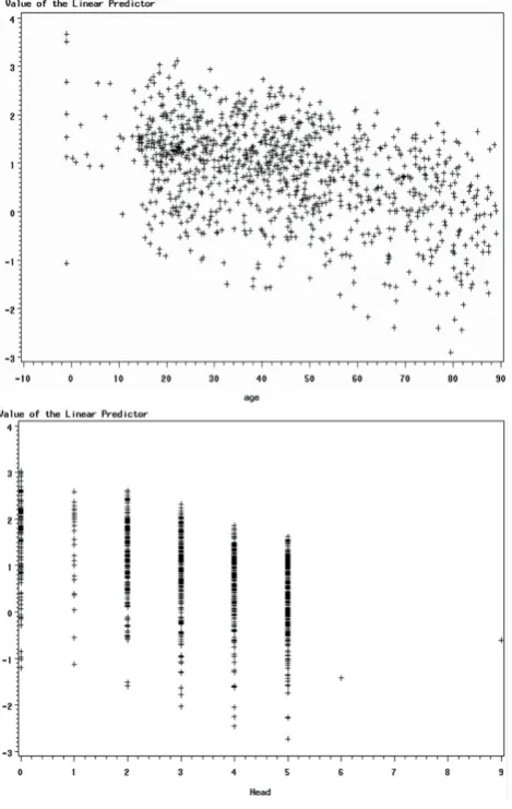
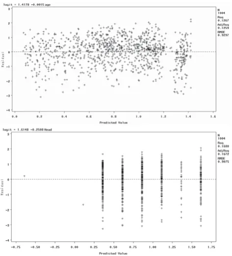
The advantage of using the logit scale for interpretation is that the relationship between the logit and the predictors is linear. To check this linearity assumption, we used scatter plot and residual analysis. The results showed linear relationships for all variables, though some were weaker than others. In the interests of brevity, in this paper we present the results for only two variables: Head AIS and Age. First, we present the scatter plot between the logit and its predictor, and then the residual plot between them using regression analysis. If the linearity assumption is satisfied, we would expect the residuals to vary randomly – i.e. they would not demonstrate any pattern. If the residual plot appears to form a curve, there may be a nonlinear relationship in the variable. This analysis was performed using statistical analysis software (SAS). Figure 1 and Figure 2 present the scatter plots and residual plots using Age and Head AIS as the predictors for patient survival.
If the plots of the residuals versus the predictors do show curvature, a quadratic term should be tested for statistical significance for suggesting better model. If the coefficient for this quadratic term is significant, the quadratic term should be included. Even though our model does not show any strong curvature, we test the Head AIS variable using a quadratic term, to validate our results. The model is as follows:
logit=a+bx +gx2 (11)
where a is an intercept term, b is a parameter of the predictor, and g is a parameter of squared predictor. For the Head AIS variable, the estimate of b is -0.1820 (p value = 0.0015), and the estimate of g is -0.0124 (p value = 0.2058). These p values indicate that Head AIS does not require a quadratic term; therefore, there is a linear relationship between the logit and its predictor.
To test the significance of the individual variables, we compare a reduced model that drops one of the
independent variables with a full model using log likelihood test. The likelihood ratio test itself does not tell us if any particular independent variables are more important than others. However, by estimating the maximum likelihood, we can analyze the difference between results for the full model and results for a nested reduced model which drops one of the indepen-dent variables. A non-significant difference indicates no effect on performance of the model, hence we can justify dropping the given variable. We call this directed MLE.
The test takes the ratio of the maximized value of the likelihood function for the full model (L1) over the Figure 1
maximized value of the likelihood function for the simpler model (L0). The resulting likelihood ratio is
given by:
−2 0 = − − = − −
1
2 0 1 2 0 1
log(L ) [log( ) log( )] ( )
L L L L L (12)
If the chi-square value for this test is significant, the variable is considered to be a significant predictor. Following these tests, only the significant variables (p value <= .05) are selected.
Note that forward and stepwise model selections are also available to discover the significance of individual attributes [19, 25]. In the literature of statistical regres-sion, the stepwise method is commonly used to find the best subset of variables for outcome prediction, con-sidering all possible combinations of variables. How-ever, the stepwise approach may not guarantee that the most significant variables are selected due to the repetition of insertion and deletion. For example, age may not be selected as important variable; however,
physicians may believe that patient age is important in deciding treatment. Therefore, we prefer to use directed MLE for our medical application. Our other justification for using MLE is empirical; in our previous study [10], we found that the direct MLE method has slightly higher accuracy in finding significant variables than stepwise and forward model selection. A statistical analysis tool, in this case SAS, is used to calculate the significance of individual attributes.
Constructing reliable rules
As mentioned previously, SVM and neural networks do not directly produce grammatical rules; therefore, only CART and C4.5 are considered for rule extraction. Those variables identified as significant are used as input variables to CART and C4.5. Also, if a rule is created only to accommodate one or two examples, it may be too specific to be applied to the entire population. Consequently, only the rules with both high accuracy and a sufficiently large number of supporting examples are used to form the rule base. Note that SVM, Neural Networks and AdaBoost are still tested in the interests of performance comparision, even though they do not generate rules. These algorithms are in widespread use, and comparing them to the rule based CART and C4.5 algorithms tests and validates the accuracy and stability of the rule-based system.
Results
The average accuracy of survival prediction without any knowledge of pre-existing conditions is 73.9%, rising to 75.8% when this knowledge is included. The off-site dataset is therefore used for further prediction tests, as it contains records of pre-existing conditions. We discov-ered that knowledge of these conditions appears at the highest level of the tree when using CART and C4.5, indicating their potential importance in the decision-making process. In particular, coagulopathy (bleeding disorder), which can result in severe haemorrhage, may be among the most important factors to consider in patients with TBI.
Due to the transparent nature of the rule-based system used in this study, the generated rules can not only help trauma experts predict the likelihood of survival, but also provide the reasoning behind these predictions in order to help physicians better allocate their resources.
Since the total number of examples used for training is rather small, initially only rules with at least 85% prediction accuracy on the testing sets are included in the rule base. This threshold was chosen following discussion with trauma experts. However, we also incorporate rules with accuracy between 75% and 85%.
Figure 2
There are two reasons for this. Firstly, the accuracy of a rule may be low due to the lack of of a truly complete database, rather than a flaw in the rule itself. Secondly, even though a rule may have low accuracy, it might include knowledge of hidden relationships between variables. For example, most trauma experts consulted believed that a patient with an ISS score over 25 would have little chance of survival. However, the survival probability might be higher for a patient with a high ISS score, but lower head and thorax AIS score, provided appropriate and prompt treatment is provided. There-fore, we will use those rules with accuracy between 75% and 85% as additional "supporting rules" in suggesting possible treatment. This issue is addressed further in the discussion section.
Significant variable selection
In order to improve the rule quality and accuracy, it is essential that we identify the key variables in the dataset. In addition, shorter rules that are based on fewer, more significant variables are more clinically useful for physi-cians. Direct MLE with logistic regression is used to
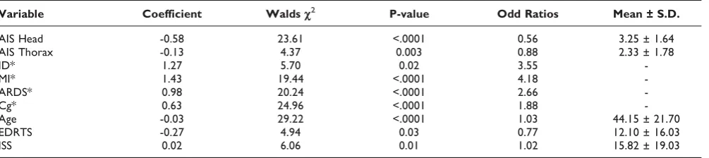
accurately extract these key variables from our helicopter and off-site datasets; the results for the off-site dataset are presented in Table 4. It can be seen that nine important variables are identified. Using standard deviations, Wald chi-squares are computed on each variable and the odd ratios are interpreted as showing a strong relationship between the outcome and the independent variables. Table 5 presents the significant variables extracted from the helicopter dataset. Only five of the eleven original variables are identified as significant.
In this study the scale of the data is small and several variables are unknown, so participating physicians assisted in identifying significant variables. These physi-cians selected age, GCS, blood pressure, pulse rate, respiration rate, and airway as important factors.
Measuring performance
The prediction results of five different machine learning methods are compared in Table 6. The performance for all algorithms is clearly superior when only significant variables are used. In addition, using only the most
Table 4: Significant variables of off-site dataset
Variable Coefficient Waldsc2 P-value Odd Ratios Mean ± S.D.
AIS Head -0.58 23.61 <.0001 0.56 3.25 ± 1.64
AIS Thorax -0.13 4.37 0.003 0.88 2.33 ± 1.78
ID* 1.27 5.70 0.02 3.55
-MI* 1.43 19.44 <.0001 4.18
-ARDS* 0.98 20.24 <.0001 2.66
-Cg* 0.63 24.96 <.0001 1.88
-Age -0.03 29.22 <.0001 1.03 44.15 ± 21.70
EDRTS -0.27 4.94 0.03 0.77 12.10 ± 16.03
ISS 0.02 6.06 0.01 1.02 15.82 ± 19.03
Categorical variables are starred. Cg stands for Coagulapathy; MI for Myocardial Infarction; ARDS for Acute Respiratory Distress Syndrome; ID for Insulin Dependent; EDRTS for Emergency Department Revised Trauma Score; ISS for Injury Severity Score.
Table 5: Significant Variables of Helicopter dataset
Variable Coefficient Walsc2 P-value Odd Ratios Mean ± S.D.
Age -0.02 3.17 <.0001 0.98 31.79 ± 17.50
Blood Pressure 0.01 2.85 0.01 0.01 129.45 ± 30.51
ISS-HN 0.01 0.003 0.25 1.11 3.22 ± 1.00
ISS -0.14 36.47 0.02 0.87 19.56 ± 11.09
ISS stands for Injury Severity Score; ISS-HN for Head/Neck Injury Severity Score.
Table 6: Performance comparison of five machine learning methods
Logistic AdaBoost C4.5 CART SVM RBF NN
All Variables 69.4% 70% 68% 75.6% 73% 67.2%
Significant Vars. only 72.9% 73% 75.2% 77.6% 79% 79.04%
significant variables is shown to result in a more balanced testing-training performance. Discussion with physicians revealed that generated recommendations and predictions must be transparent in their reasoning; our system therefore uses CART and C4.5 to predict patient survival. If physicians understand the reasoning behind decisions and it follows their own, their confidence in the system may be increased. If the system's reasoning is clinically meaningless, they can choose to disregard the recommendation; however, if the reasoning has some clinical merit, this may alert them to previously hidden factors affecting patient outcome.
Table 7 presents the performance accuracy in outcome prediction (rehabilitation or home) for the off-site dataset, and prediction of ICU days for the helicopter dataset. In both cases, only the significant variables are used. No attempt is made to use all available variables, since the survival prediction test has already confirmed the improved performance when using only significant variables.
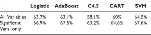
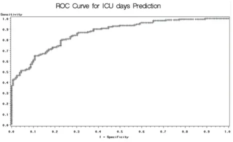
We also generate Receiver Operating Characteristic (ROC) curves –plots of the true positive rate (sensitiv-ity) versus the false positive rate (1-specific(sensitiv-ity)–in order to evaluate the model performance. First, we perform ROC analysis on the patient surivival prediction results. Table 8 compares the area under the curve (AUC) for the ROC curves generated using all available variables and significant-only variables. The table shows that results are improved when using only significant variables in the model. Therefore, when dealing with the helicopter dataset, we only perform ROC analysis on the signifi-cant-variable-only model. The results are presented in Table 9. Notice that there is no large difference in ROC analysis results among the various machine learning methods. However, when the dataset is small– such as our data used for ICU days prediction – logistic regression outperforms the other methods. Figure 3 and Figure 4 present sample ROC plots for logistic regression using only significant variables for survival and ICU days prediction respectively.
Constructed database using CART and C4.5
Numerous rules were generated with the CART and C4.5 rule extraction algorithm. Following discussion with trauma
Table 7: Prediction results for outcome and ICU days
Logistic AdaBoost C4.5 CART SVM RBF NN
Exact Outcome 74.6% 73% 75.6% 72% 72.6% 72.8%
Days in ICU 80.6% 78.7% 77.1% 77.4% 80.1% 77.4%
This table compares the performance of logistic regression alone and the five chosen machine learning algorithms in predicting exact outcome (for off-site dataset) and ICU length of stay (for helicopter dataset).
Table 8: Performance comparison of AUC in ROC curve analysis
Logistic AdaBoost C4.5 CART SVM
All Variables 63.7% 63.1% 58.1% 60% 64.5%
Significant Vars. only
66.9% 67.5% 63.2% 64.6% 67.6%
Table 9: ROC performance in Exact outcome and ICU days predictions
Variable Logistic AdaBoost C4.5 CART SVM
Exact out-come
76.8% 76.4% 71.9% 71.5% 68.7%
Days in ICU 79.2% 74.6% 76.6% 73% 71.9%
Figure 3
experts, we identified the robust rules as those with over 85% accuracy. For survival prediction, the average rule accuracy using all available variables is 82%, and 83.9% when using only the most significant variables.
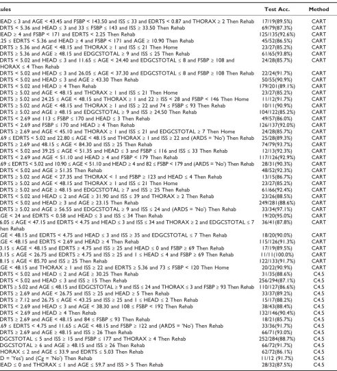
Table 10 presents the most reliable generated rules for survival prediction (> 85% accuracy); Table 11 contains
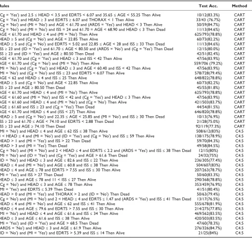
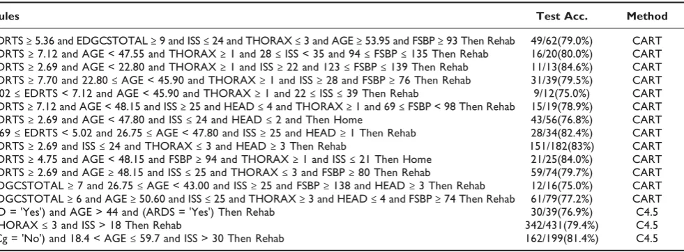
survival rules with accuracy between 75% and 85%. Similarly, Table 12 presents the most reliable generated rules for outcome prediction (> 85% accuracy), and Table 13 contains outcome rules with accuracy between 75% and 85%. Finally, Table 14 presents the most reliable generated rules for ICU days predic-tion (> 85% accuracy), and Table 15 contains ICU days rules with accuracy between 75% and 85%. Note that the rules with accuracy between 75% and 85% may not be sufficiently reliable, yet may contain useful pattern information, as described in the discussion section.
Discussion
We developed a computer-aided rule-base using signifi-cant variables selected via logistic regression, and showed that the approximations of the variables help increase rule quality. Our intent is to extract and formulate medical diagnostic knowledge into an appro-priate set of transparent decision rules that can be used in a computer-assisted decision making system. The proposed method extracts the most significant variables using logistic regression with direct maximization like-lihood estimation. By comparing the performances using five machine learning algorithms – AdaBoost, C4.5, CART, RBF neural network, and SVM–using all available
Figure 4
ROC plot for Logistic regression on ICU days prediction. This figure presents the ROC plot obtained when applying logistic regression for ICU days prediction, using only significant variables.
Table 10: Extracted reliable rules for survival prediction (> 85% accuracy)
Rules Test Accuracy Method
(Cg = 'Yes') and HEAD < 2 and AGE < 76.65 Then Alive 29/34(85.3%) CART
(Cg = 'No') and (MI = 'No') and AGE < 61.70 and HEAD≤4 and (ARDS = 'No') Then Alive 334/375(89.1%) CART
(Cg = 'No') and (MI = 'No') and HEAD≥5 and AGE < 22.35 Then Alive 55/64(85.9%) CART
ISS≥28 and (Cg = 'No') and THORAX≤4 and 62.25≤AGE < 69.00 and EDRTS≥2.88 Then Alive 10/11(90.9%) CART
ISS≥23 and (Cg = 'No') and THORAX≤4 and 69≤AGE < 72.35 Then Alive 13/15(86.7%) CART
HEAD≤2 and (MI = 'No') and (Cg = 'No') and AGE≤62 Then Alive 182/206(88.3%) C4.5
(MI = 'Yes') and AGE≤62 and EDRTS > 5.39 and ISS≤25 Then Alive 19/20(95%) C4.5
THORAX > 3 and HEAD≤4 and (ARDS = 'No') and AGE≤62 Then Alive 126/148(85.1%) C4.5
THORAX≤2 and EDRTS≤0.87 and ISS > 38 Then Dead 12/13(92.3%) C4.5
(MI = 'Yes') and AGE > 82.6 Then Dead 16/18(88.9%) C4.5
(MI = 'Yes') and ISS > 30 Then Dead 45/50(90%) C4.5
HEAD > 4 and (MI = 'Yes') Then Dead 25/27(92.6%) C4.5
(Cg = 'Yes') and HEAD≤4 and AGE > 78 Then Dead 12/14(85.7%) C4.5
(ID = 'Yes') and AGE > 78 and (MI = 'Yes') and HEAD≤4 Then Dead 27/31(87.1%) C4.5
HEAD > 0 and HEAD≤2 and (ID = 'Yes') and (ARDS = 'No') and AGE≤75.2 Then Alive 107/118(90.7%) C4.5
(ID = 'Yes') and (MI = 'Yes') and HEAD > 3 Then Dead 43/49(87.8%) C4.5
(MI = 'Yes') and (ID = 'Yes') and AGE > 78 Then Dead 32/37(86.5%) C4.5
HEAD > 4 and (MI = 'Yes') Then Dead 25/27(92.6%) C4.5
(MI = 'Yes') and ISS > 30 Then Dead 45/50(90%) C4.5
(MI = 'Yes') and AGE > 79.6 and ISS > 12 Then Dead 27/30(90%) C4.5
(Cg = 'Yes') and HEAD≤4 and AGE > 79.6 Then Dead 12/14(85.7%) C4.5
(ARDS = 'No') and (MI = 'No') and (Cg = 'No') and HEAD≤4 and AGE≤62 Then Alive 335/376(89.1%) C4.5
(MI = 'Yes') and (ID = 'Yes') and AGE > 78 Then Dead 15/16(93.8%) C4.5
(MI = 'Yes') and HEAD≤4 and ISS > 38 Then Dead 29/34(85.3%) C4.5
(MI = 'Yes') and AGE≤61.6 and ISS > 27 Then Dead 26/30(86.7%) C4.5
HEAD = 2 and (MI = 'No') and AGE≤62 and ISS≤38 Then Alive 235/270(87%) C4.5
THORAX > 0 and (ID = 'Yes') and ISS≤30 Then Alive 13/14(92.9%) C4.5
variables and significant variables only, we found that using only the most significant variables provides a considerable improvement in performance. All five methods show improvement across all-available and significant-variables-only, indicating that our proposed selection method is robust and efficient.
The performance of individual rules was measured; reliable rules were identified as those with accuracy above 85%. In addition, all rules we selected were
considered reliable if the number of cases in the dataset matching the rule was higher than a specified threshold. Rule sensitivity and specificity were also measured, and the average sensitivity and specificity for the three outcome pairs (alive/dead, home/read, severe/ non-severe) are 87.4% and 88.4% respectively. This indicates that our method performs well. Some addi-tional improvements may be needed to improve rule quality. In particular, large and well balanced datasets across all outcome classes could improve overall quality, Table 11: Extracted supporting rules for survival prediction (75%–85% accuracy)
Rules Test Acc. Method
(Cg = 'Yes') and 2.5≤HEAD < 3.5 and EDRTS < 6.07 and 35.65≤AGE < 55.25 Then Alive 10/12(83.3%) CART
(Cg = 'Yes') and HEAD≥3 and EDRTS≥6.07 and THORAX < 1 Then Alive 33/43 (76.7%) CART
(Cg = 'No') and (MI = 'No') and AGE < 61.70 and (ARDS = 'Yes') and HEAD < 3 Then Alive 50/59(84.7%) CART
(Cg = 'No') and (MI = 'No') and ISS = 24 and 61.70 = AGE < 68.90 and HEAD≤3 Then Dead 11/13(84.6%) CART
AGE < 61.70 and HEAD≤4 and (MI = 'No') Then Alive 625/793(78.8%) CART
HEAD≥5 and (Cg = 'No') and AGE < 22.85 Then Alive 60/73(82.2%) CART
HEAD≥5 and (Cg = 'No') and EDRTS < 5.02 and 22.85≤AGE < 28 and ISS≥33 Then Dead 11/13(84.6%) CART
ISS≥23 and (ID = 'Yes') and 61.70≤AGE < 80.50 and (ARDS = 'No') and (Cg = 'Yes') Then Dead 12/15(80.0%) CART
ISS≥23 and (ID = 'Yes') and AGE≥80.50 Then Dead 42/51(82.4%) CART
AGE < 61.70 and (Cg = 'Yes') and HEAD≤3 and ISS < 42 Then Alive 47/56(83.9%) CART
AGE < 61.70 and (Cg = 'No') and (MI = 'No') Then Alive 559/706 (79.2%) CART
(MI = 'No') and (Cg = 'Yes') and HEAD≤3 and AGE < 60.40 and ISS < 42 Then Alive 47/56(83.9%) CART
(MI = 'No') and (Cg = 'No') and ISS≤23 and EDRTS < 6.07 Then Alive 578/728(79.4%) CART
AGE < 62 and HEAD≤4 and ISS≤25 Then Alive 648/822(78.8%) CART
HEAD≥5 and (Cg = 'No') and AGE < 22.85 Then Alive 60/73(82.2%) CART
ISS≥23 and AGE≥80.50 Then Dead 45/55(81.8%) CART
AGE < 61.70 and HEAD≤4 and (MI = 'No') Then Alive 625/793(78.8%) CART
AGE < 61.60 and (MI = 'No') and ISS < 42 and (Cg = 'Yes') and HEAD≤3 Then Alive 47/56(83.9%) CART
AGE < 61.60 and HEAD≤4 and (MI = 'No') and (Cg = 'No') Then Alive 421/503(83.7%) CART
AGE≥61.60 and ISS≥23 and (Cg = 'Yes') Then Dead 44/54(81.5%) CART
AGE < 61.70 and HEAD≤4 and (ISS < 27) Then Alive 646/820(78.8%) CART
HEAD≥5 and (Cg = 'No') and 22.35≤AGE < 25.85 and (MI = 'No') and ISS≥30 Then Dead 10/13(76.9%) CART
ISS≥23 and 61.70≤AGE < 74.10 and EDRTS < 2.88 Then Dead 21/28(75.0%) CART
ISS≥23 and AGE≥74.10 Then Dead 92/119(77.3%) CART
(MI = 'No') and HEAD≤4 and AGE≤62 ISS≤38 Then Alive 508/612(83%) C4.5
3 < HEAD≤4 and (MI = 'No') and (ID = 'Yes') and (Cg = 'No') and ISS≤59 Then Alive 138/175(78.9%) C4.5
HEAD > 1 and (MI = 'Yes') and ISS > 22 Then Dead 59/70(84.3%) C4.5
HEAD > 3 and (MI = 'Yes') Then Dead 49/58(84.5%) C4.5
(Cg = 'No') and (MI = 'No') and 2 < HEAD≤4 and EDRTS≤2.2 and (ARDS = 'Yes') and ISS≤38 Then Dead 12/15(80%) C4.5
(MI = 'No') and (ID = 'Yes') and (Cg = 'Yes') and AGE > 61.6 Then Dead 24/32(75%) C4.5
(ID = 'No') and HEAD≤3 and AGE≤82.6 and ISS≤22 Then Alive 236/305(77.4%) C4.5
HEAD≤4 and (MI = 'No') and AGE≤60.8 and ISS≤38 Then Alive 504/607(83%) C4.5
HEAD≤4 and AGE≤78 and EDRTS > 7.55 and ISS≤30 Then Alive 207/263(78.7%) C4.5
(MI = 'Yes') and ISS > 27 Then Dead 50/60(83.3%) C4.5
HEAD≤3 and AGE≤78 and 11 < ISS≤27 Then Alive 290/368(78.8%) C4.5
(Cg = 'No') and HEAD≤3 and AGE≤78 Then Alive 353/459(76.9%) C4.5
(MI = 'Yes') and EDRTS≤5.39 Then Dead 41/51(80.4%) C4.5
HEAD > 0 and (MI = 'Yes') and THORAX > 2 and (ID = 'No') Then Dead 50/63(79.4%) C4.5
(Cg = 'No') and (MI = 'No') and 2 < HEAD≤4 and EDRTS≤1.47 and (ARDS = 'Yes') and ISS≤41 Then Dead 13/17(76.5%) C4.5
HEAD≤4 and (MI = 'No') and AGE≤62 and ISS≤41 Then Alive 555/678(81.9%) C4.5
HEAD≤4 and AGE≤79.6 and EDRTS > 7.55 and ISS≤30 Then Alive 214/275(77.8%) C4.5
(MI = 'No') and HEAD≤4 and AGE≤61.6 and ISS≤34 Then Alive 469/562(83.5%) C4.5
HEAD≤3 and AGE≤61.6 and ISS≤38 Then Alive 420/503(83.5%) C4.5
(MI = 'Yes') and (ID = 'Yes') and AGE > 68.5 Then Dead 47/60(78.3%) C4.5
(ARDS = 'No') and HEAD≤3 and AGE≤61.9 Then Alive 276/326(84.7%) C4.5
(ID = 'No') and (MI = 'Yes') and EDRTS > 5.39 and ISS≤14 Then Alive 21/25(84%) C4.5
Table 12: Extracted reliable rules for outcome prediction (> 85% accuracy)
Rules Test Acc. Method
HEAD≤3 and AGE < 43.45 and FSBP < 143.50 and ISS≤33 and EDRTS < 0.87 and THORAX≥2 Then Rehab 17/19(89.5%) CART
EDRTS < 5.36 and HEAD≤3 and 33≤FSBP≤143 and ISS≥33.50 Then Rehab 69/79(87.3%) CART
HEAD≥4 and FSBP < 171 and EDRTS < 2.25 Then Rehab 125/135(92.6%) CART
2.25≤EDRTS < 5.36 and HEAD≥4 and FSBP < 171 and AGE≥10.90 Then Rehab 45/52(86.5%) CART
EDRTS≥5.36 and AGE < 48.15 and THORAX≥1 and ISS≤21 Then Home 23/27(85.2%) CART
EDRTS≥5.36 and AGE≥48.15 and EDGCSTOTAL≥9 and ISS≤25 Then Rehab 61/65(93.8%) CART
EDRTS < 5.02 and HEAD≤3 and 11.65≤AGE < 24.40 and EDGCSTOTAL≤8 and FSBP≥108 and
THORAX≤4 Then Rehab
24/28(85.7%) CART
EDRTS < 5.02 and HEAD≤3 and 26.05≤AGE < 37.30 and EDGCSTOTAL≤8 and FSBP≥108 Then Rehab 22/24(91.7%) CART
EDRTS < 5.02 and HEAD≤3 and AGE≥43.30 Then Rehab 50/55(90.9%) CART
EDRTS < 5.02 and HEAD≥4 Then Rehab 179/201(89.1%) CART
EDRTS≥5.02 and AGE < 48.15 and THORAX≥1 and ISS≤21 Then Home 23/27(85.2%) CART
EDRTS≥5.02 and 24.25≤AGE < 48.15 and THORAX≥1 and 22≥ISS < 28 and FSBP < 146 Then Home 11/12(91.7%) CART
EDRTS≥5.02 and AGE < 48.15 and THORAX≥1 and ISS≥22 and 74≤FSBP≤93 Then Rehab 10/11(90.9%) CART
EDRTS≥5.02 and AGE≥48.15 and EDGCSTOTAL≥9 and ISS≥24.50 Then Rehab 104/122(85.2%) CART
EDRTS < 2.69 and 113≤FSBP≤170 and HEAD≤3 Then Rehab 49/57(86.0%) CART
EDRTS < 2.69 and FSBP≤170 and HEAD≥4 Then Rehab 126/137(92.0%) CART
EDRTS≥2.69 and AGE < 45.10 and THORAX≥1 and ISS≤21 and EDGCSTOTAL≥7 Then Home 24/28(85.7%) CART
2.69≤EDRTS < 5.02 and 22.80≤AGE < 48.15 and THORAX≥1 and ISS≥22 and (ARDS = 'No') Then Rehab 25/28(89.3%) CART
EDRTS≥2.69 and 48.15≤AGE < 84.30 and ISS≥25 Then Rehab 74/79(93.7%) CART
EDRTS < 5.02 and 39.25≤AGE < 51.35 and HEAD≤3 and FSBP≤116 and ISS≤33 Then Rehab 12/13(92.3%) CART
EDRTS < 2.69 and AGE < 51.10 and HEAD≥4 and FSBP < 179 Then Rehab 117/126(92.9%) CART
2.69≤EDRTS < 5.02 and 10.90≤AGE < 51.10 and HEAD≥4 and 82≤FSBP < 179 and (ARDS = 'No') Then Rehab 28/31(90.3%) CART
EDRTS < 5.02 and AGE≥51.35 Then Rehab 48/52(92.3%) CART
EDRTS≥5.02 and AGE < 27.35 and THORAX < 1 and FSBP≥123 and HEAD≤4 Then Rehab 13/15(86.7%) CART
EDRTS≥5.02 and AGE < 48.15 and THORAX≥1 and ISS≤21 Then Home 23/27(85.2%) CART
EDRTS≥5.02 and AGE≥48.15 and EDGCSTOTAL≥7 and ISS≥25 Then Rehab 61/66(92.4%) CART
EDRTS < 5.02 and HEAD≤2 and AGE≥31.90 and ISS≤39 and THORAX≥2 Then Rehab 23/26(88.5%) CART
EDRTS < 5.02 and HEAD≥3 and AGE≥23.15 Then Rehab 249/281(88.6%) CART
EDRTS≥5.02 and AGE≥56.55 and EDGCSTOTAL≥9 and ISS≤24 and (ARDS = 'No') Then Rehab 33/34(97.1%) CART
AGE < 24 and EDRTS < 0.58 and HEAD≤3 and ISS≤34 Then Rehab 19/20(95.0%) CART
26.05≤AGE < 47.15 and EDRTS < 4.75 and HEAD≤3 and ISS≤34 and THORAX≥2 and EDGCSTOTAL≤7
Then Rehab
36/41(87.8%) CART
AGE < 48.15 and EDRTS < 4.75 and HEAD≤3 and ISS≥35 and EDGCSTOTAL≤7 Then Rehab 18/20(90.0%) CART
AGE < 48.15 and EDRTS < 2.69 and HEAD≥4 Then Rehab 115/126(91.3%) CART
23.15≤AGE < 48.15 and EDRTS≥4.75 and ISS≥25 and HEAD≤0 and FSBP≥69 Then Rehab 17/19(89.5%) CART
23.15≤AGE < 26.75 and EDRTS≥4.75 and ISS≥25 and 1≤HEAD≤4 and FSBP≥69 Then Rehab 11/11(100.0%) CART
48.15≤AGE < 85.70 and ISS≥25 Then Rehab 122/133(91.7%) CART
AGE < 48.15 and THORAX≥1 and ISS≥22 and EDRTS≥5.36 and 73≤FSBP < 120 Then Home 20/22(90.9%) CART
EDRTS < 5.02 and HEAD≤2 and AGE≥30.25 Then Rehab 31/35(88.6%) C4.5
EDRTS < 5.02 and HEAD≤3 and ISS≥15 Then Rehab 256/294(87.1%) C4.5
EDRTS≥5.02 and AGE≤48.15 and EDGCSTOTAL≥9 and ISS≤24 and THORAX≤3 and FSBP≥93 Then Rehab 110/127(86.6%) C4.5
EDRTS≥2.69 and AGE < 26.75 and ISS≥25 and HEAD≥5 Then Rehab 33/37(89.2%) C4.5
EDRTS≥7.12 and 26.75≤AGE < 43.25 and ISS≥25 and 1≤HEAD≤2 Then Rehab 15/17(88.2%) C4.5
EDRTS < 2.69 and HEAD≤3 and AGE < 38.30 and 108≤FSBP < 192 Then Rehab 38/43(88.4%) C4.5
EDRTS < 2.69 and HEAD≥4 Then Rehab 132/146(90.4%) C4.5
EDRTS≥2.69 and AGE < 48.15 and 84≤FSBP≤93 Then Rehab 18/21(85.7%) C4.5
2.69≤EDRTS < 4.75 and 11.65≤AGE < 48.15 and FSBP≥122 and (ARDS = 'No') Then Rehab 33/36(91.7%) C4.5
EDRTS≥2.69 and AGE≥48.15 and ISS≥26 Then Rehab 66/71(93.0%) C4.5
EDGCSTOTAL≤5 and ISS≥15 and FSBP≤177 and THORAX≥4 Then Rehab 252/284(88.7%) C4.5
EDGCSTOTAL≥6 and AGE≥48.15 and ISS≥26 Then Rehab 66/72(91.7%) C4.5
THORAX≤2 and AGE≤33.9 and EDRTS≤5.03 Then Rehab 62/72(86.1%) C4.5
(ID = 'Yes') and (Cg = 'No') Then Rehab 11/12 (91.7%) C4.5
HEAD≤0 and THORAX≤1 and AGE≤59.7 and ISS > 5 Then Rehab 28/32(87.5%) C4.5
as well as sensitivity and specificity. Full sensitivity and specificity results for the datasets are presented in Table 16.
One important issue in rule selection is how to deal with rules with accuracy below 85%. When using only the over-85% rules, some medical knowledge in the data-base might have been ignored. The accuracy of a rule may be low due to the lack of "database completeness", rather than a flaw in the rule itself. Therefore, rules with less than 85% accuracy cannot be completely removed from the rule based system. We will instead use those rules as additional "supporting rules" in suggesting possible treatment. For example, according to trauma experts, patients with a high ISS score (> 25) are least likely to survive. However, we found some rules with surprising implications. For instance, one of these "counterintuitive" rules pointed to the fact that there are 52 alive cases (3.3%) with ISS high scores (38). Of these 52 patients, 33 (63.5%) have high AIS head scores (≥4), and 38 patients (73%) are male. Considering the above conditions, surviving patients have lower thorax (average score = 2.61) and lower abdomen AIS scores (average score = 1.03) than fatal cases. These fatal cases typically have a higher head AIS score (average score = 5.08) than surviving patients (average head score = 3.90). In addition, we found that none of the surviving patients have complications such as coagulopathy, and only a few had a pre-existing disease (in particular, Insulin Dependency and Myocardial Infarction).
While only Acute Respiratory Distress Syndrome (ARDS) is usually considered an impact factor in predicted survival, according to the created rules, pre-existing conditions, Acute Respiratory Distress Syndrome (ARDS), Insulin Dependency, Myocardial Infarction, and Coagulopathy all have significant impact. Also, airway status (need/not need) was identified as a primary factor in predicting the number of ICU days for patients transported via helicopter.
Note that for ICU length of stay prediction, 74.6% of patients stayed at in ICU less than 2 days. Only 25.4% of patients stayed more than 2 days, and only 2.9% of those were in ICU for more than 20 days. This reinforces Eckhart's point that many patients are transported via helicopter unnecessarily. Therefore, the use of accurate ICU days prediction rules may help improve the efficiency of helicopter transport, considering cost effectiveness as well as the treatment of patients in critical condition.
Conclusion
The results in this paper provide a framework to improve the physicians' diagnostic accuracy with the aid of machine learning algorithm. The resulting system is effective in predicting patient survival, and rehab/home outcome. A method has been introduced that creates a variety of reliable rules that make sense to physicians by combining CART and C4.5 and using only significant Table 13: Extracted supporting rules for outcome prediction (75%–85% accuracy)
Rules Test Acc. Method
EDRTS≥5.36 and EDGCSTOTAL≥9 and ISS≤24 and THORAX≤3 and AGE≥53.95 and FSBP≥93 Then Rehab 49/62(79.0%) CART
EDRTS≥7.12 and AGE < 47.55 and THORAX≥1 and 28≤ISS < 35 and 94≤FSBP≤135 Then Rehab 16/20(80.0%) CART
EDRTS≥2.69 and AGE < 22.80 and THORAX≥1 and ISS≥22 and 123≤FSBP≤139 Then Rehab 11/13(84.6%) CART
EDRTS≥7.70 and 22.80≤AGE < 45.90 and THORAX≥1 and ISS≥28 and FSBP≥76 Then Rehab 31/39(79.5%) CART
5.02≤EDRTS < 7.12 and AGE < 45.90 and THORAX≥1 and 22≤ISS≤39 Then Rehab 9/12(75.0%) CART
EDRTS≥7.12 and AGE < 48.15 and ISS≥25 and HEAD≤4 and THORAX≥1 and 69≤FSBP < 98 Then Rehab 15/19(78.9%) CART
EDRTS≥2.69 and AGE < 47.80 and ISS≤24 and HEAD≤2 and Then Home 43/56(76.8%) CART
2.69≤EDRTS < 5.02 and 26.75≤AGE < 47.80 and ISS≥25 and HEAD≥1 Then Rehab 28/34(82.4%) CART
EDRTS≥2.69 and ISS≤24 and THORAX≤3 and HEAD≥3 Then Rehab 151/182(83%) CART
EDRTS≥4.75 and AGE < 48.15 and FSBP≥94 and THORAX≥1 and ISS≤21 Then Home 21/25(84.0%) CART
EDRTS≥2.69 and AGE≥48.15 and ISS≤25 and THORAX≤3 and FSBP≥80 Then Rehab 59/74(79.7%) CART
EDGCSTOTAL≥7 and 26.75≤AGE < 43.00 and ISS≥25 and FSBP≥138 and HEAD≥3 Then Rehab 12/16(75.0%) CART
EDGCSTOTAL≥6 and AGE≥50.60 and ISS≤25 and THORAX≥3 and HEAD≤4 and FSBP≥74 Then Rehab 61/79(77.2%) CART
(ID = 'Yes') and AGE > 44 and (ARDS = 'Yes') Then Rehab 30/39(76.9%) C4.5
THORAX≤3 and ISS > 18 Then Rehab 342/431(79.4%) C4.5
(Cg = 'No') and 18.4 < AGE≤59.7 and ISS > 30 Then Rehab 162/199(81.4%) C4.5
variables extracted via logistic regression. The resulting computer-aided decision-making system has significant benefits, both in providing rule-based recommendations and in enabling optimal resource utilization. This may ultimately assist physicians in providing the best possible care to their patients. The diagnosis of future patients may also be improved by analyzing all possible rules associated with their symptoms.
The system will be tested at all 17 hospitals of the Carolinas Healthcare System (CHS). Software that provides the computer-aided decision making system will be optimized and made available to the academic community as a web-based application, as well as a software tool on portable personal computing devices. Feedback from every hospital will then be considered and used to validate and improve the system.
Competing interests
The authors declare that they have no competing interests.
Authors' contributions
TH is responsible for obtaining the data and providing feedback on the medical impact of the results. SJ, RS and KN have designed the algorithms, analyzed the data, and drafted the manuscript. All authors have equal participa-tion in the study as well as preparaparticipa-tion of the final paper.
Acknowledgements
This research was partially funded by research grants from Health Services Foundation, Carolinas HealthCare System, and Virginia Commonwealth University. This material is based upon work supported by the National Science Foundation under Grant No.IIS0758410. The authors would like to thank these institutions for their support.
Table 14: Extracted reliable rules for ICU days prediction (> 85% accuracy)
Rules Test Acc. Method
(AIRWAY = 'Need') and 115≤ED-BP < 156 and AGE≥47.05 and Then ICU stay days≥3 14/15(93.3%) CART
(AIRWAY = 'Need') and 115≤ED-BP < 156 and ED-RESP < 18 and 4.35≤AGE < 14.5 Then ICU stay days≥3 12/12(100%) CART
(AIRWAY = 'No Need') and ED-RESP≥21 and 45≤AGE < 55.85 Then ICU stay days≤2 10/11(90.1%) CART
(AIRWAY = 'Need') and ED-BP < 91 Then ICU stay days≥3 14/14(100%) CART
(AIRWAY = 'Need') and 93.5≤ED-BP < 156.5 and ED-PULSE≥60.5 and AGE≥54.2 Then ICU stay days≥3 10/10(100%) CART
(AIRWAY = 'Need') and 94≤ED-BP < 156 and ED-PULSE≥61 and ED- RESP < 19 and 18.45≤AGE < 44.5 Then ICU stay days≥3
60/76(86.6%) CART
(AIRWAY = 'No Need') and AGE < 52.9 and ED-BP≥107 and ED- GCS≥11 Then ICU stay days≤2 175/192(91.1%) CART
(AIRWAY = 'Need') and ED-BP < 150.5 and ED-RESP < 19 and AGE≥4.9 and ED-PULSE≥138 Then ICU stay days≥3
18/20(90%) CART
(AIRWAY = 'Need') and ED-RESP < 19 and ED-PULSE < 138 and ED- BP < 115 and 10.9≤AGE < 47.3 Then ICU stay days≥3
31/33 (93.9%) CART
(AIRWAY = 'No Need') and AGE < 37.1 and ED-GCS≥11 and ED- BP≥125 Then ICU stay days≤2 89/90(98.9%) CART
(AIRWAY = 'No Need') and AGE < 37.1 and ED-GCS≥11 and ED- BP < 119 Then ICU stay days≤2 39/44(88.6%) CART
(AIRWAY = 'No Need') and AGE < 37.1 and ED-GCS≥13 and 119≤ED- BP < 125 and ED-PULSE≥90
Then ICU stay days≤2
21/22(95.5%) CART
(AIRWAY = 'Need') and 146≤ED-BP < 156 and AGE < 22.5 Then ICU stay days≥3 11/12(91.2%) CART
(AIRWAY = 'No Need') and AGE < 37.05 and ED-GCS≥9 Then ICU stay days≤2 157/172(91.3%) CART
(AIRWAY = 'No Need') and 37.05≤AGE < 46.9 and ED-RESP < 21 and ED-PULSE < 121 Then ICU stay days≤2 23/25(92%) CART
(AIRWAY = 'No Need') and ED-RESP < 21 and ED-PULSE < 121 and AGE≥49.7 and ED-BP≥141
Then ICU stay days≤2
12/13(92.3%) CART
(AIRWAY = 'No Need') and AGE < 37.05 and ED-GCS < 10 and 114≤ED- BP < 142 Then ICU stay days≤2 11/12(91.7%) CART
(AIRWAY = 'Need') and ED-BP < 91.5 Then ICU stay days≥3 14/14(100%) CART
(AIRWAY = 'Need') and 91≤ED-BP < 156 and 95.5≤ED-PULSE < 102.5 Then ICU stay days≥3 15/17(88.2%) CART
(AIRWAY = 'No Need') and AGE < 52.9 and ED-BP≥99 and ED- GCS≥13 Then ICU stay days≤2 177/196(90.3%) CART
(AIRWAY = 'No Need') and ED-BP < 134 and 37.05≤AGE < 67.35 and ED-RESP < 19 Then ICU stay days≤2 11/12(91.7%) CART
(AIRWAY = 'Need') and ED-PULSE≥62 and AGE≥24.35 and ED- BP < 110 Then ICU stay days≥3 26/29(89.7%) CART
(AIRWAY = 'Need') and 110≤ED-BP < 180 and ED-PULSE≥62 and 47.05≤AGE < 68.2 Then ICU stay days≥3 16/17(94.1%) CART
(AIRWAY = 'No Need') and AGE < 37 and ED-GCS≥13 Then ICU stay days≤2 147/159(92.5%) CART
(AIRWAY = 'No Need') and AGE≥37 and 135≤ED-BP < 163 Then ICU stay days≤2 26/29(89.7%) CART
(AIRWAY = 'Need') and ED-PULSE≥62 and AGE≥24.35 and ED- BP < 110 Then ICU stay days≥3 31/35(88.6%) CART
(AIRWAY = 'Need') and ED-BP < 91 Then ICU stay days≥3 14/14(100%) CART
(AIRWAY = 'Need') and 93≤ED-BP < 156 and ED-RESP < 19 and AGE≤54.05 Then ICU stay days≥3 10/10(100%) CART
(AIRWAY = 'Need') and ED-RESP < 19 and 93≤ED-BP < 119 and 18.45≤AGE < 47.3 Then ICU stay days≤3 24/26(92.3%) CART
(AIRWAY = 'No Need') and ED-GCS≥11 and ED-BP≥88 and AGE < 37.05 Then ICU stay days≤2 148/160(92.5%) CART
Age≤42 and (Airway = 'No Need') and ED-PULSE≤137 and ED- RESP > 19 Then ICU stay days≤2 100/116(86.2%) C4.5
Age > 37 and ED-BP≤95 Then ICU stay days≥3 14/14(100%) C4.5
References
1. Anderson RN, Minino AM, Fingerhut LA, Warner M, Heinen MA and Eds:Deaths: Injuries, 2001.National Vital Statistics Reports2001,52 (21):1–87.
2. Centres for Disease Control and Prevention:Facts about Concussion and Brain Injury and Where to Get Help. Atlanta, GA2004.
3. The Coalition for American Trauma. http://www.traumacoali-tion.org.
4. Expert Working Group:Traumatic Brain Injury in the United States: Assessing Outcomes in Children. Atlanta, GA2000.
5. Fabian TC, Patton JH, Croce MA, Minard G, Kudsk KA and Pritchard FE: Blunt carotid injury: Importance of early diagnosis and anticoagulant therapy. Ann Surg 1996, 223 (5):513–525.
6. Jagielska I:Linguistic rule extraction from neural networks for descriptive data mining. Proc. 2nd Int'l Conf. Knowledge-Based Intelligent Electronic Systems: 21–23 Apr 1998, Adelaide1998, 89–92. 7. Arfken CL, Shapiro MJ, Bessey PQ and Littenberg B:Effectiveness of Helicopter versus Ground Ambulance Services for Interfacility Transport.Journal of Trauma-Injury Infection & Critical Care1998,45(4):785–790.
8. Cunningham P, Rutledge R, Baker CC and Clancy TV: A comparison of the association of helicopter and ground ambulance transport with the outcome of injury in trauma patients transported from the scene. J Trauma 1997, 43 (26):940–946.
9. Ruggieri S:Efficient C4.5.IEEE Trans on Knowl and Data Eng2002,
14(2):438–444.
10. Ji SY, Huynh T and Najarian K: An intelligent method for computer-aided trauma decision making system.ACM-SE 45: Proceedings of the 45th annual southeast regional conference2007, 198– 202.
11. Gearhart PA, Wuerz R and Localio AR: Cost-effectiveness analysis of helicopter EMS for trauma patients. Ann Emerg Med1997,30(4):500–506.
12. Eckstein M, Jantos T, Kelly N and Cardillo A: Helicopter Transport of Pediatric Trauma Patients in an Urban Emergency Medical Services System: A Critical Analysis.J Trauma2002,53(2):340–344.
13. Haug PJ, Gardner RM and Tate KE: Decision support in medicine: examples from the HELP system. Comput Biomed Res1994,27(5):396–418.
14. Fitzmaurice JM, Adams K and Eisenberg JM: Three Decades of Research on Computer Applications in Health Care: Medical Informatics Support at the Agency for Healthcare Research and Quality.Journal of the American Medical Informatics Association2002,9(2):144–160.
15. Quinlan J: Improved use of continuous attributes in C4.5. Journal of Artificial Intelligence Research1996,4:77–90.
16. Clarke JR, Hayward CZ, Santora TA, Wagner DK and Webber BL:
Computer-generated trauma management plans: compar-ison with actual care.World J Surg2002,26(5):536–538.
Table 15: Extracted supporting rules for ICU days prediction (75%–85% accuracy)
Rules Test Acc. Method
(AIRWAY = 'No Need') and ED-RESP < 21 and ED-BP < 142 ED- PULSE < 79 and 37.05≤AGE < 44.15 Then ICU stay days≤2
13/16(81.3%) CART
(AIRWAY = 'No Need') and AGE≥52.9 and ED-BP≥141 Then ICU stay days≤2 12/15(80%) CART
(AIRWAY = 'Need') and 117≤ED-BP < 135 and ED-RESP < 19 and 68≤ED-PULSE < 138 and 15.05≤AGE < 46.4 Then ICU stay days≥3
23/28(82.1%) CART
(AIRWAY = 'Need') and 136≤ED-BP < 150 and ED-RESP < 19 and ED-PULSE < 138 and 15.05≤AGE < 23.25 Then ICU stay days≥3
10/13(77%) CART
(AIRWAY = 'No Need') and 96≤ED-BP < 163 and 39.15≤AGE < 69.05 Then ICU stay days≤2 44/55(80%) CART
(AIRWAY = 'Need') and ED-BP < 156 and AGE≥24.35 Then ICU stay days≥3 76/96(79.2%) CART
(AIRWAY = 'Need') and ED-BP < 146 and AGE < 17.85 and 135≤ED-PULSE < 181 Then ICU stay days≥3 9/11(81.2%) CART
(AIRWAY = 'Need') and ED-BP < 146.5 and AGE < 17.85 and ED- PULSE < 131 and ED-RESP < 18 Then ICU stay days≥3
15/20(75%) CART
(AIRWAY = 'No Need') and ED-BP≥141 Then ICU stay days≤2 223/265(84.2%) CART
(AIRWAY = 'Need') and ED-BP < 114 Then ICU stay days≥3 44/52(84.6%) CART
(AIRWAY = 'Need') and 114≤ED-BP < 135.5 and ED-PULSE < 97 and 17.2≤AGE < 46.95 and ED-RESP < 7 Then ICU stay days≥3
10/13(77%) CART
(AIRWAY = 'No Need') and AGE≥52.9 and ED-BP≥141 Then ICU stay days≤2 12/15(80%) CART
(AIRWAY = 'Need') and ED-BP < 114 Then ICU stay days≥3 44/52(84.6%) CART
(AIRWAY = 'Need') and 110.5≤ED-BP < 180.5 and ED- PULSE≥62 and 4.35≤AGE < 44.5 and ED-GCS < 10 Then ICU stay days≥3
35/46(76.1%) CART
(AIRWAY = 'No Need') and AGE≥37 and 135≤ED-BP < 163 Then ICU stay days≤2 31/35(88.6%) CART
(AIRWAY = 'No Need') and 37.05≤AGE < 55.6 and ED-GCS≥11 and 88≤ED-BP < 163 Then ICU stay days≤2 40/49(81.6%) CART
ED-BP > 100 and ED-RESP > 19 Then ICU stay days≤2 145/180(80.6%) C4.5
Though these rules are not reliable enough for practical use, they can contain pattern information which may be of interest to physicians. ED-BP is Emergency Department Blood Pressure; RESP is Emergency Department Respiratory Rate; PULSE is Emergency Department Pulse Rate; ED-GCS is Emergency Department Glasgow Coma Score.
Table 16: Rule sensitivity and specificity
Off-site Dataset Off-site Dataset Helicopter Dataset
Predictive Outcome Alive/Dead Home/Rehab ICU stay Days
Sensitivity (> 85% rules) 91.9% 88.7% 90.6%
Specificity (> 85% rules) 89.2% 87.7% 91%
Sensitivity (75%–85% rules) 86.2% 79% 82.5%