Modelling Filler Dispersion in Elastomers: Relating
Filler Morphology to Interface Free Energies via
SAXS and TEM Simulation Studies
Norman Gundlach and Reinhard Hentschke*
School of Mathematics and Natural Sciences, Bergische Universität, D-42097 Wuppertal, Germany; [email protected] (N.G.)
* Correspondence: [email protected]; Tel.: + 49-202-439-2628
Abstract: The properties of rubber are strongly influenced by the distribution of filler within the polymer matrix. Here we introduce a Monte Carlo-based morphology generator. The basic elements of our model are cubic cells, which, in the current version, can be either silica filler particles or rubber volume elements in adjustable proportion. The model allows the assignment of surface free energies to the particles according to whether a surface represents, for instance, ’naked’ silica or silanised silica. The amount of silanisation is variable. We use a nearest-neighbour site-exchange Monte Carlo algorithm to generate filler morphologies, mimicking flocculation. Transmission electron micrographs (TEM) as well as small angle scattering (SAS) intensities can be calculated along the Monte Carlo trajectory. In this work we demonstrate the application of our morphology generator in terms of selected examples. We illustrate its potential as a tool for screening studies, relating interface tensions between the components to filler network structure as characterized by TEM and SAS.
Keywords:elastomers; lattice model; Monte Carlo simulation; surface tensions; small angle scattering; transmission electron microscopy
1. Introduction
Polymer nanocomposites, i.e. polymer matrices containing nanoparticles of variable amounts and types, posses a broad range of applications [1]. In particular, nanofillers are standard ingredients of rubber compounds, most often added to improve mechanical toughness [2]. Because their relative amounts are rather high, the addition of filler does generally influence all properties - mechanical and others - to a significant extend. This also means that the addition of filler, its chemistry and processing alike, can be used to adjust the material properties. Our focus is on rubber in tyre applications, where filler is added primarily as reinforcing agent (e.g. [3]). It nevertheless affects other properties like rolling resistance, grip or wear (e.g. [4]). One key parameter in this context is dispersion [5].
Dispersion of filler involves the application of shear-forces to distribute filler uniformly in a polymer matrix. There are different levels of dispersion distinguished as visual, macro- and micro-dispersion. We concentrate on the latter - specifically on the dispersion ranging from primary particles over aggregates to the filler network on the scale of up to 1µm. Even when the filler is uniformly dispersed in the elastomer matrix, the filler particles will tend to flocculate in the post-mixing stages like storage, extrusion or vulcanization [6–11] (simular structural developments can also be observed in other contexts like drying of polymer nanocomposites [12]). Our modelling approach to this phenomenon, discussed in the following, is driven by local equilibrium thermodynamics in conjunction with the interface tensions between the various components.
Experimentally different methods are employed to asses the dispersion of filler in a rubber matrix depending on the type of dispersion (e.g. [4]). In the case of micro-dispersion transmission electron microscopy (TEM), atomic force microscopy and small angle X-ray (SAXS) or neutron (SANS) scattering techniques are used - either individually or in combination (e.g. [13–15]). In the following our focus will be on the combination of TEM with SAXS.
Nanofillers in polymer matrices have been studied extensively using molecular dynamics (MD), Monte Carlo (MC) and related computer simulation techniques. Quantities of interest encompass polymer density profiles, polymer and polymer segment mobility, the effect of particles on the glass transition temperature or the system’s viscosity. A comprehensive overview is given in a recent article by Hagita et al. [16]. In the same reference the authors study a particularly large system of≈2000 nanoparticles embedded in≈40000 chains consisting of≈1000 beads each. They compare two fixed nanoparticle configurations (dispersed vs. aggregated) when the simulation box is stretched. These large simulations involve quite rough coarse grained interaction potentials and are limited to very short times. A different type of simulation approach to the structure formation in nano-composites is described by Martin [17]. The studies described in this reference, as well as in the references therein, focus on the effects of grafted chains on the effective force between model nanoparticles in effective solvents and polymer melts. Yet another concept is developed in Ref. [18]. Structural information obtained via transmission electron microscopy and scattering methods is used to construct filler network structures, whose elastic properties are then investigated. Nevertheless, it was noted recently by Legters et al. [19] that there still is a large gap in our understanding of the complex hierarchical structures in the actual multi-component nano-composites in industrial applications. The focus of this work therefore is the dependence of the filler structure or morphology on the actual interfacial tensions of the real components, which is outside the usual quantities of interest mentioned above. An exception is the recent work by Stöckelhuber et al. [20]. They study filler flocculation in polymers in a simplified model derived from game theory, where nevertheless the interactions are based on interface free energies derived from thermodynamics. We shall return to this work below.
At the usual filler concentrations (volume fraction 10 to 20%), the dispersed aggregates have some contact with each other. These contacts play in important role in the pronounced non-linearity exhibited by the dynamic moduli of filled elastomers (Payne effect). In previous work we have modelled the contribution of single inter particle contacts in filler networks to energy dissipation, rolling resistance in particular [21], as well as reinforcement based on the chemical composition of the system [22]. Application of this approach on the macroscopic scale, particularly to the relation between molecular composition and dynamic moduli, requires information regarding the number of filler contacts along a load bearing network path (cf. [23]) and, generally speaking, the morphology of the network as a whole.
In this work we discuss a filler morphology generator based on a coarse-grained description of the ingredients in conjunction with measured interface or surface tensions. We employ a nearest-neighbour site-exchange MC algorithm, where the transition probabilities are based on experimental interface tensions between three components (polymer, silica and silane), to model filler dispersion on the micro-scale. The basic elements of our model are cubic cells, which can be either silica filler particles or rubber volume elements. The model allows the assignment of different surface free energies to the particles according to whether a surface represents, for instance, ’naked’ silica or silanised silica. The amount of silanisation is variable. Aside from the aforementioned motivation, the proposed morphology generator is useful for screening purposes, relating surface energies to filler structure.
2. Materials and Methods
2.1. Monte Carlo Flocculation
polymer - filler network
lattice model (polymer not
shown)
filler particle
m nm
coarse-graining
TESPT
Figure 1.Hierarchy of scales. The polymer matrix within an elastomer composite, here exemplified by a tyre tread material, is reinforced by an embedded filler network. In the current model the filler particles are approximated by cells on a cubic lattice (coarse graining). The different coloured faces are either representing bare particle surface areas (blue) or silanised areas (red). A specific example are silica particles silanised with TESPT.
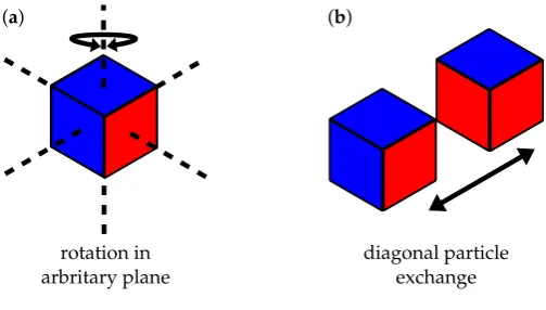
We model the flocculation process employing two local MC moves as depicted in Fig. 2. The first move consists of the random selection of a lattice cell and its subsequent rotation by a random multiple ofπ/2 with respect to a likewise random axis of the lattice. Subsequently a nearest-neighbour site exchange move interchanges two diagonal neighbour cells. Again the pair to be exchanged is picked randomly. Note that these particular moves are chosen, because they can be implemented quite efficiently. Each move separately is followed by a Metropolis criterion, i.e
min(1, exp[β∆W]≥ξ. (1)
Hereβ−1=kBT, wherekBis Boltzmann’s constant andTis the temperature. In additionξis a random number between zero and unity. If this inequality is satisfied, then the respective move is accepted.
rotation in
arbritary plane diagonal particleexchange
(a) (b)
Figure 2.Illustration of MC moves. (a) Particle (cube) rotation; (b) Neighbouring particle exchange.
The quantity∆Wis obtained as follows. The equilibrium free enthalpyGof the system is given by
G= ∑iGie
−βGi
∑ie−βGi
MC Step at room temperature
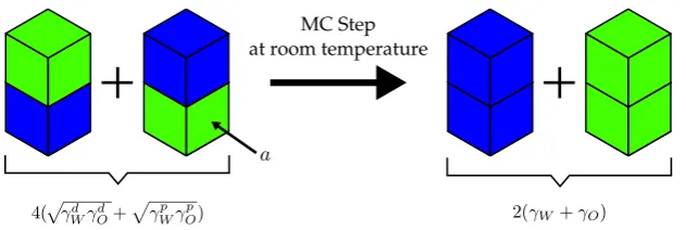
Figure 3.Example MC step in a water-oil mixture as explained in the text. The neighbouring particle exchange step is performed at room temperature, i.e.kBT=2.48kJ/mol. The interfacial area for each type of interface isa.
The quantitiesGidenote the free enthalpies at fixed configurationsi. Note that this simply follows fromβG=−lnQNPTtogether withQNPT=∑iQi,NPT =∑ie−βGi in conjunctionG= N∂G/∂Nand
Gi=N∂Gi/∂N(extensivity). Also at equilibrium
dG|T,P,Nk=γjdAj. (3)
HerePis the pressure in the system, and Nkis number of cells of typek. γj denotes the interface tension of a face-to-face pairing of typejand Aj = njadenotes the attendant total area of j-type interfaces in the system. Note thatais the effective contact area per face, which we assume to be the same for allj. Notice also that we use the summation convention. The proper∆W, for a system developing towards equilibrium underNPT-conditions, therefore is given by∆W =−γj∆Aj, i.e.
exp[β∆W] =exp−β γja∆nj . (4)
This generates system configurations satisfying Eq. (2) on average. Away from equilibrium the algorithm will drive the system towards the lowest possible free enthalpyGand the number of MC moves should be a rough measure of time. This may be justified by the local nature of the moves in conjunction with the assumption of a local equilibrium. The latter is commonly invoked during the derivation of transport equations in the framework of non-equilibrium thermodynamics [24].
2.2. Surface Tensions
Our thermodynamic modelling approach to flocculation is different from the game-theoretical algorithm proposed in Ref. [20]. However, as the authors of Ref [20], we also model the particle-to-particle interaction in terms of interface tensions. The interface tensionsγjare expressed via the approximation
γj ≡γαβ=γα+γβ−2
q γαdγdβ+
q γαpγ
p β
(5)
Note thatγα =γαd+γ p
α. The same applies toγβof course. Here the superscriptsdandpindicate the dispersive and polar part of the surface tensions ofαorβ. Notice that a detailed discussion of this equation can be found in Ref. [25]. In addition, all numerical values for the surface tensions used in the following examples, unless stated otherwise, are taken from this work.
∆W =−γja∆nj =−γwwa−γooa+2γwoa. (6) Inserting Eq. (5) we find
∆W=2a
γw+γo−2(
q γdwγdo+
q γpwγop)
. (7)
If we now use the values γdw = 13.1 kJ/(mol·nm2), γwp = 30.7 kJ/(mol·nm2) and γdo = 18.9 kJ/(mol·nm2),γp
o =0.96 kJ/(mol·nm2) (olive oil) [26] we find at room temperature, i.e.kBT =2.48 kJ/mol,
β∆W≈17anm−2 (8)
This means that this particular MC step is accepted - regardless of what the concrete size ofais. In the following we use experimental surface tensions obtained from literature sources.
2.3. Calculation of TEM pictures and SAXS intensities
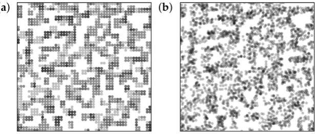
Transmission electron micrograph images are generated from slices, 5 cells thick, extracted from the system after a certain number of MC steps. An example is shown in the left panel of Fig.4. Grey circles correspond to filler cells on the lattice. The shading becomes darker when filler cells are stacked along the line of sight. In order to increase the similarity to experimental TEM slices it is useful to apply small random displacements to the circles. The maximum displacement in any direction is 0.6 times the lattice spacing (Note that the same procedure precedes the calculation of scattering intensities.). Applying this to the aforementioned slice in Fig.4, we obtain the right panel.
(
a
)
(
b
)
Figure 4.Mock TEM picture generation. (a) A slice, thickness 5 particle diameters, is extracted from the simulation after a certain number of MC steps; (b) Small random displacements, as described in the text, are applied to every particle in the slice. Darker spots are due to two or more particles superimposed along the line of sight.
In addition to the TEM images based on slices, we can compute the SAXS intensity based on the entire simulation box (see also [27]). The total intensity is the product of two factors, i.e.
FP(q)∝
(
S q−4 q→∞
V2 q→0 . (10)
HereS =4πR2andV =4πR3/3 are the surface and the volume of the particles, respectively. The q−4-behaviour is known as Porod’s law [28]. For particles possessing a fractal surface structure, characterised by a surface fractal exponentds, one can show [29] that Porod’s law is replaced byq−6+ds. The cross-over from one limit to another occurs in a narrow regime aroundqR = π. This means that scattering intensity above the particular value ofqis essentially constant and does not affect the q-dependence of the total intensity in this range. The latter is governed bySa/n(q), which is due to aggregated particles and the filler network in general. We expressFP(q)in terms of an approximation due to Beaucage [30], combining the laws of Guinier and Porod, which is approximately valid over the entireq-range, i.e.
FP(q) =∆ρ2
V2exp[−q2R2/5] +2πSq∗−4 . (11) Note that q∗ = q/(erf(qR/√10))3 and ∆ρ is the contrast difference between filler and polymer. Realistic filler particles are polydisperse. Therefore R is the mean particle size of the attendant distribution andFP(q)is the corresponding average intensity.
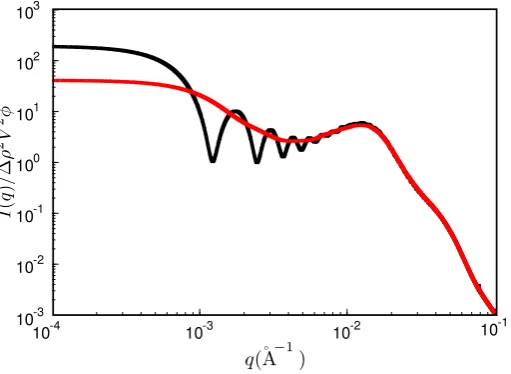
Figure 5.Reduced scattered intensity vs. magnitude of the scattering vector,q. Black: result obtained from a single MC configuration generated in a cubic box with periodic boundaries; red: result obtained after the averaging procedure explained in the text.
The structure factorSa/n(q), on the other hand, is given by
Sa/n(q) =φ
1+4πρ Z ∞
0 drr 2sinqr
qr (g2(r)−1)
. (12)
We use 30 to 50 such boxes varying in size between 100% to 18% inL, whereL3is the volume of the original box. The result is the red curve in Fig.5. Note that the curve now is much more smooth, but the intensity is reduced in the smallqlimit. We return to this point below.
It is worth noting that the underlying length scales in Eqs. (11) and (12) are conceptually different. The length scale in Eq. (11) isR, whereas in Eq. (12) it is the lattice spacing,a. The simplest choice, which also yields the best results, amounts to settingR=a.
3. Results
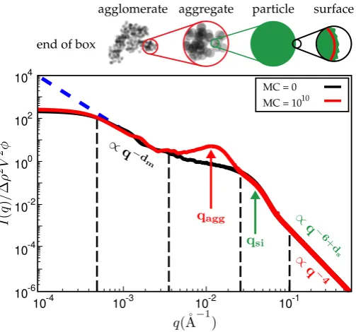
Figure6is a typical plot of reduced intensity vs.qobtained at different stages of the MC. In the limit of smallqthe intensity is governed entirely byFP(q)and thus is not affected by the MC at all. The average diameter of the primary filler particles, here≈2π/qSi, is an input parameter and allows to expressqin units of a specific inverse length. The strongest effect is due to formation of aggregates during the MC, leading to a peak which characterises the average aggregate diameter (≈2π/qagg). Theq-range labeled∝q−dmin Fig.6reflects the super-structure beyond the aggregates. We expect this
structure to be characterised by its mass fractal dimensiondm, i.e. the intensity in this regime should be∝q−dm. The close to homogeneous initial filler distribution yieldsdm=3. If the mixing produces a
fractal network we expect smaller values. The problem is that the attendantq-range should be at least an order of magnitude wide. This requires quite large system sizes of up to 108cells in our case. Ifq becomes very small, the box size eventually is exceeded and the scattering intensity levels off.
MC = 0 MC = 1010 end of box
agglomerate aggregate particle surface
Figure 6. Reduced scattered intensity vs. magnitude of the scattering vector,q. The figure depicts the differentq-regimes. The limit of largeqis governed by Porod’s law or, in the case of fractal particle surfaces, by the attendant law exhibiting a fractal dimension. Subsequentq-regimes contain information on the size of the particles, their aggregates and the filler network itself. Due to the finite size of the simulation cell, there is a plateau terminating useful information at smallq. The observed structure of course depends on the number of MC steps.
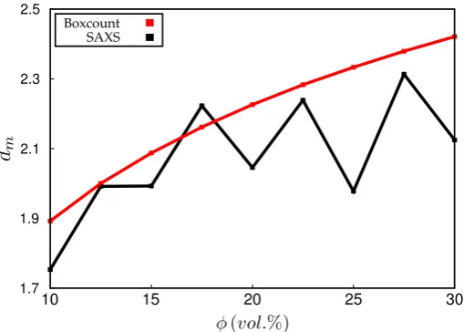
the system is partitioned inton3cells. Whenever a cell contains at least one particle it is considered occupied. Plotting the logarithm of the number of occupied cells, lnAn, vs. lnn, should yield a slope equal todmfor sufficiently largen. Figure7compares the values ofdmobtained by both methods for systems containing different amounts of filler. Notice that the system size is quite large in this case, i.e. the lattice dimension is 256×256×256. The numerical uncertainty of both methods is comparable, even though the box-counting algorithm appears to be smooth. The averaging over boxes of different size, as explained in the context of Fig.5, tends to reduce the slope of the scattering intensity in the q-regime wheredmis determined. This is why the box-counting algorithm yields somewhat large values for the fractal dimension. In a recent work by Mihara et al. [15] the authors study flocculation in silica-filled rubber using small-angle X-ray measurements. Their fractal dimensions tend to be larger than the ones obtained here. For instance, using the conventional silica VN3, theirdmincreases from about 2.6 to 2.7 when the silica content increases from 60 to 80 phr. This corresponds roughly toφbetween 0.15 and 0.2 in our case and thus the increase at least is comparable. Nevertheless, it is difficult to compare this conclusively, because the general system compositions differ.
Boxcount SAXS
Figure 7.Mass fractal dimension,dm, vs. filler volume fraction,φ. Black:dmcalculated from fits to the scattering intensity in the range 5·10−4<q<4·10−3; red:d
mcalculated via box-counting algorithm. Note that the system studied here forφ=0.25 is identical to the systems in Fig.4and Fig.6.
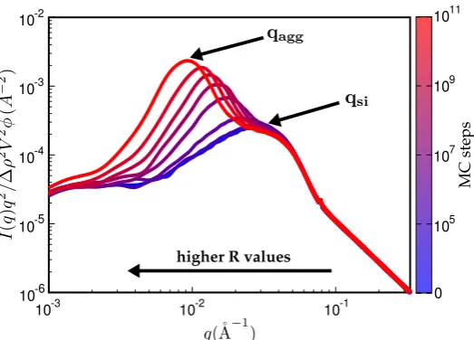
In the following we discuss a number of examples illustrating the approach. In order to study aggregate formation it is useful to multiply the scattering intensity by an extra factorq2(Kratky-plot). Figure8shows the reduced intensity using this Kratky-representation. Notice that the height of the aggregate peak increases and also shifts to smallerq-values with increasing number of MC steps. At the beginning of the MC only the particle-peak is present. Subsequently the MC generates continuously growing aggregates for this particular system.
higher R values
MC steps
Figure 8. Kratky representation of the scattering intensity vs. qfor different number of MC steps. Increasing number of MC steps shifts the aggregate peak atqaggto smaller qvalues, resulting in growing aggregates. The particle peak atqsiremains at its position.
aggregate
particle particle
aggregate
(a) (b)
Figure 9.Approximate comparison between simulation and experiment. (a) Kratky representation of the scattered intensity obtained via simulation after 1010MC steps on a 256×256×256 lattice. The system consists of polybutadiene rubber (BR, Lanxess Buna CB25) and precipated silica (Ultrasil VN3, granulated form). The silanes are represented by using TESPT surface modified Ultrasil VN3, i.e. Coupsil 8113. The mean particle size quoted in the literature ishRi=80 Å. Filler volume fraction is
φ=7.5 %. The aggregate size corresponding to the aggregate peak is about 202 Å. (b) Experimental
scattering curve taken from Ref. [14] for styrene-butadiene rubber (SBR) filled with Zeosil 1165 MP. Filler volume fraction isφ=8.4 %. The particle and aggregate sizes according to the attendant peaks
are 139 Å and 402 Å, respectively. HereT=160◦C.
the course of the indicated number of MC steps small aggregates do form in BR. Their characteristic size is slightly larger than twice the size of the primary particles.
Aerosil 200
Ultrasil VN3 gran.
8 10 Ultrasil VN3 gran.
Aerosil 200
MC steps
(a)
(b)
Figure 10.(a) Simulated TEM images. (b) Attendant simulated SAXS curves. The rubber is CR (Lanxess Baypren) at 80 % (by volume) and the silane is again represented by Coupsil 8113 with a content of 5 % (by volume) in both systems. Each system is either filled with 15 % Ultrasil VN3 gran. atT=433 K (right TEM and dashed SAXS curves) or, alternatively, with Aerosil 200.
CR
BR
8 10 BR
CR
MC steps
(a)
(b)
Figure 11.(a) Simulated TEM images. (b) Attendant simulated SAXS curves. Here the filler is Ultrasil VN3 gran., as in one of the systems in the previous figure. The rubber is alternatively BR or CR.
4. Discussion
the relevant interface tensions. TEM images and attendant SAXS curves are calculated along the trajectory, allowing the comparison to corresponding experimental systems. Due to the local character of the MC steps we can, albeit in a rough sense, relate the flocculation kinetics to the number of MC steps. The present simulations are for systems containing three components, i.e. elastomer, filler, and coupling agent. However, addition of extra components is straightforward. Most rubbers for example, utilise elastomer blends. A second type of elastomer is added easily via an additional cube type. The entire approach is computationally cheap, unless the goal is the large scale network structure - here characterised in terms of a mass fractal dimension. If the initial aggregation behaviour is sufficient, then the approach is particularly suited for screening studies. In addition the following is worth noting. System morphologies generated in the fashion described here, can be useful for as input to coarse grained models for the calculation of macroscopic dynamic moduli as for instance discussed in Refs. [31–34]. In particular, modelling the Payne effect requires information on the number of reversible filler-to-filler contacts in inside the network and, more precisely, the number of reversible filler-to-filler contacts along load-bearing path at a particular deformation state [23].
Acknowledgments:We are grateful for a number of very useful discussions with Drs. Ali Karimi-Varzaneh and Nils W. Hojdis.
Author Contributions:Norman Gundlach - computer simulations and model development, Reinhard Hentschke - study supervision, model development and drafting of the manuscript.
Conflicts of Interest:The authors declare no conflict of interest.
Abbreviations
The following abbreviations are used in this manuscript:
SA(X)S Small Angle (X-Ray) Scattering TEM Transmission Electron Microscopy MC Monte Carlo
BR polybutadiene rubber CR polychloroprene rubber
References
1. Kumar, S.K.; Benicewicz, B.C.; Vaia, R.A.; Winey, K.I. 50th Anniversary Perspective: Are Polymer Nanocomposites Practical for Applications? Macromolecules2017,50, 714–731.
2. Leblanc, J.L.Filled Polymers: Science and Industrial Applications.; CRC Press: Boca Raton, 2010.
3. Roland, C.M. Reinforcement of Elastomers. InReference Module in Materials Science and Materials Engineering; Elsevier, 2016.
4. Nikiel, L.; Gerspacher, M.; Yang, H.; O’Farrell, C.P. Filler Dispersion, Network Density, and Tire Rolling Resistance. Rubber Chemistry and Technology2001,74, 249–259.
5. Lacayo-Pineda, J. Filler Dispersion and Filler Networks. InEncyclopedia of Polymeric Nanomaterials; Springer: Berlin, 2014.
6. Vilgis, T.A.; Heinrich, G.; Klüppel, M.Reinforcement of Polymer Nano-Composites; Cambridge University Press: New York, 2009.
7. Böhm, G.G.A.; Nguyen, M.N. Flocculation of Carbon Black in Filled Rubber Compounds. 1. Flocculation Occurring in Unvulcanized Compounds During Annealing at Elevated Temperatures. J. Appl. Polym. Sci. 1995,55, 1041–1050.
8. Lin, C.J.; Hergenrother, W.L.; Alexanian, E.; Böhm, G.G.A. On the Filler Flocculation in Silica-Filled Rubbers Part I. Quantifying and Tracking the Filler Flocculation and Polymer-Filler Interactions in the Unvulcanized Rubber Compounds.Rubber Chem. Technol.2002,75, 865–890.
9. Mihara, S.; Datta, R.N.; Noordermeer, J. Flocculation in Silica Reinforced Rubber Compounds. Rubber Chem. Technol.2009,82, 524–540.
11. Robertson, C.G. Flocculation in Elastomeric Polymers Containing Nanoparticles: Jamming and the New Concept of Fictive Dynamic Strain. Rubber Chem. Technol.2015,88, 463–474.
12. Kim, S.; Hyun, K.; Ahn, B.S.K.H.; Clasen, C. Structural Development of Nanoparticle Dispersion during Drying in Polymer Nanocomposite Films. Macromolecules2016,49, 9068–9079.
13. Jouault, N.; Vallat, P.; Dalmas, F.; Said, S.; Jestin, J.; Boue, F. Well-Dispersed Fractal Aggregates as Filler in Polymer-Silica Nanocomposites: Long-Range Effects in Rheology.Macromolecules2009,42, 2031–2040. 14. Baeza, G.P.; Genix, A.C.; Degrandcourt, C.; Petitjean, L.; Gummel, J.; Couty, M.; Oberdisse, J. Multiscale
Filler Structure in Simplified Industrial Nanocomposite Silica/SBR Systems Studied by SAXS and TEM. Macromolecules2013,46, 317–329.
15. Mihara, S.; Datta, N.; Dierkes, W.K.; Noordermeer, J.W.M.; Amino, N.; Ishikawa, Y.; Nishitsuji, S.; Takenaka, M. Ultra Small-Angle X-Ray Scattering Study of Flocculation in Silica-Filled Rubber.Rubber Chem. Technol. 2014,87, 348–359.
16. Hagita, K.; Morita, H.; Doi, M.; Takano, H. Coarse-Grained Molecular Dynamics Simulation of Filled Polymer Nanocomposites under Uniaxial Elongation. Macromolecules2016,49, 1972–1983.
17. Martin, T.B. Entropic and Enthalpic Driving Forces on Morphology in Polymer Grafted Particle Filled Nanocomposites. PhD thesis, University of Colorado at Boulder, Boulder, Colorado, 2016.
18. Jean, A.; Willot, F.; Cantournet, S.; Forest, S.; Jeulin, D. Large-Scale Computations of Effective Elastic Properties of Rubber with Carbon Black Fillers.Intl. J. Multiscale Computational Engineering2011,9, 271–303. 19. Legters, G.; Kuppa, V.; Beaucage, G.; University of Dayton Collaboration.; University of Cincinnati
Collaboration. Coarse-Grained Simulation of Polymer-Filler Blends. APS March Meeting Abstracts, 2017, p. M1.083.
20. Stöckelhuber, K.W.; Wießner, S.; Das, A.; Heinrich, G. Filler Flocculation in Polymers - a Simplified Model Derived from Thermodynamics and Game Theory. Soft Matter2017,13, 3701–3709.
21. Meyer, J.; Hentschke, R.; Hager, J.; Hojdis, N.W.; Karimi-Varzaneh, H.A. A Nano-Mechnical Instability as Primary Contribution to Rolling Resistance. Scientific Reports2017,7, 11275.
22. Meyer, J.; Hentschke, R.; Hager, J.; Hojdis, N.W.; Karimi-Varzaneh, H.A. Molecular Simulation of Viscous Dissipation due to Cyclic Deformation of Silica-Silica Contact in Filled Rubber. Macromolecules2017, 50, 6679–6689.
23. Hentschke, R. The Payne Effect Revisited. Express Polymer Letters2017,11, 278–292.
24. Glandorff, P.; Prigogine, I.Thermodynamic Theory of Structure, Stability and Fluctuations; Wiley and Sons: London, 1971.
25. Stöckelhuber, K.W.; Das, A.; Jurk, R.; Heinrich, G. Contribution of Physico-Chemical Properties of Interfaces on Dispersibility, Adhesion and Flocculation of Filler Particles in Rubber. Polymer2010,51, 1954–1963. 26. Michalski, M.C.; Desobry, S.; Pons, M.N.; Hardy, J. Adhesion of Edible Oils to Food Contact Surfaces.
Journal of the American Oil Chemists’ Society1998,75, 447–454.
27. Schneider, G.J. Analyse der Struktur von Aktiven Füllstoffen mittels Streumethoden. PhD thesis, Universität Regensburg, Regensburg, 2006.
28. Glatter, O.; Kratky, O., Eds. Small Angle X-Ray Scattering; Academic Press: NewYork, 1982.
29. Bale, H.D.; Schmidt, P. Small-Angle X-Ray-Scattering Investigation of Submicroscopic with Fractal Properties. Phys. Rev. Lett.1984,53, 596–599.
30. Beaucage, G. Approximations Leading to a Unified Exponential/Power-Law Approach to Small-Angle Scattering. J. Appl. Cryst.1995,28, 717–728.
31. Long, D.; Sotta, P. Nonlinear and Plastic Behavior of Soft Thermoplastic and Filled Elastomers Studied by Dissipative Particle Dynamics.Macromolecules2006,39, 6282–6297.
32. Merabia, S.; Sotta, P.; Long, D.R. A Microscopic Model for the Reinforcement and the Nonlinear Behavior of Filled Elastomers and Thermoplastic Elastomers (Payne and Mullins Effects). Macromolecules2008, 41, 8252–8266.
33. Xi, H.; Hentschke, R. Dynamic Moduli of Filled Elastomers - A Coarse-Grained Computer Model.European Polymer Journal2012,48, 1777–1786.