www.adv-stat-clim-meteorol-oceanogr.net/1/1/2015/ doi:10.5194/ascmo-1-1-2015
© Author(s) 2015. CC Attribution 3.0 License.
Simulation of future climate under changing temporal
covariance structures
W. B. Leeds1, E. J. Moyer2, and M. L. Stein3
1Quantitative Researcher, The Climate Corporation, San Francisco, CA, USA 2Dept. of the Geophysical Sciences, The University of Chicago, Chicago, IL, USA
3Department of Statistics, University of Chicago, Chicago, IL, USA
Correspondence to: W. B. Leeds ([email protected])
Received: 4 September 2014 – Revised: 3 December 2014 – Accepted: 3 January 2015 – Published: 26 February 2015
Abstract. A growing body of evidence indicates that anthropogenic greenhouse gases are changing Earth’s climate, and that those changes may involve not only changes in climatic means but also in variability. Climate models may be informative about these future changes, but their use is complicated by the fact that they do not capture variability in current climate well. Many methods have therefore been developed to combine models and data in simulations of future climate, but current methods generally account only for changes in marginal variation and do not capture projected changes in correlation (spatial, temporal, spatiotemporal). We develop here a procedure to simulate future daily mean temperature that modifies climate observations based on changes in the mean and spectral density suggested by climate model output, and illustrate our methodology with projections from the CCSM3 (Community Climate System 3) climate model. We are able to simulate a future climate with changing temporal covariance while largely retaining non-Gaussian features of the observations. Our results suggest that in CCSM3, at most locations and most timescales, variability in daily mean temperature decreases under anthropogenic warming. The methodology presented here applies only to fully equilibrated future climate states, but may be extended to simulating transient states as well.
1 Introduction
With mounting evidence indicating that Earth’s climate is changing (IPCC, 2007, and references therein), it is becom-ing increasbecom-ingly important to understand the potential im-pacts of climate change on society. Imim-pacts assessment re-quires projections of future climate under increased concen-trations of greenhouse gases (GHGs). For example, under-standing climate effects on food supply would require simu-lations of future temperature and precipitation for use in agri-cultural yield models. Crop yields, however, are highly non-linear with temperature and precipitation and therefore are sensitive not only to climatological means but also to short-term extremes (e.g., Schlenker and Roberts, 2009; Wheeler et al., 2000). In this context, climate must be understood as an underlying, multivariate, spatiotemporal probability dis-tribution, for which weather is a random realization. Human societies can be impacted by changes of not only the mean, but of the entire probability distribution.
1900 2000 2100 2200 2300 2400 300
400 500 600 700 800
Year
CO
2
(ppm)
BASELINE SCENARIO
(a) CO2Scenarios
1900 2000 2100 2200 2300 2400 11
12 13 14 15
Temperature (
°
C)
Year
BASELINE SCENARIO DATA
OFFSET DATA
1900 2000 2100 2200 2300 2400 284 285 286 287 288
Temperature (
°
K)
(b) Annual GMT
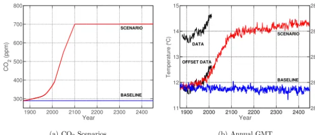
Figure 1.Comparison of modeled and observed global mean temperatures. (a) CO2concentrations used in “baseline” and “scenario” runs
with the CCSM3 model. (See Appendix A for description of experiments and observations.) Figures here truncate output after less than 600 years but the scenario run extends for 6000 years. (b) Corresponding annual model GMT (◦C) for the two runs and observed GMT from the Global Historical Climatological Network. Model output reproduces trends in global temperature well but with a systematic offset from observations. To better show the similarity in trend we also plot the observational record minus a 2◦C offset.
robust across models (see, e.g., Barnes and Polvani, 2013) or physical parameterizations (see, e.g., Hawkins et al., 2013). The area remains one of active research.
One complication to analyses of potential future changes in climate variability is that while the deterministic climate models used for long-term climate forecasts appear to cap-ture trends, they do not accurately reproduce observed cur-rent climate. These models, known as atmosphere–ocean general circulation models (AOGCMs), are physically based numerical simulations of transport of energy and moisture in the atmosphere and ocean, typically with separate submod-els for the atmosphere, ocean, sea ice, and vegetation. Many AOGCMs successfully reproduce observed large-scale cir-culation, atmospheric structure, latitudinal temperature gra-dients, storm tracks, and quasi-periodic interdecadal phe-nomena such as the El Niño–Southern Oscillation. When driven with historical records of CO2and aerosol emissions
due to human and volcanic activity, they also reproduce well the observed temperature trend of the last 2 centuries. Figure 1 demonstrates this ability to capture trends in the widely used Community Climate System 3 (CCSM3) model (Collins et al., 2006), which we use in examples throughout this manuscript. (See Appendix A for description of model and experimental runs, as well as observational data used in comparisons.) CCSM3 and other AOGCMs do not, however, perfectly reproduce either the mean or distribution of current climate. Model present-day global mean temperature (GMT) can be offset by several degrees from observations (again, see Fig. 1) and probability distributions of temperature and precipitation at individual locations do not match those of weather observations (Fig. 3, which shows marginal distri-butions in CCSM3 temperature output and observations for three representative locations whose time series are given in Fig. 2; see also Lambert and Boer, 2001, for discussion).
The comparisons above suggest that climate models may be informative about changes in climate, even while
fail-ing to capture certain current characteristics. This is well-demonstrated for means (again, see Fig. 1), and the fact that AOGCMs capture trends in mean climate well suggests that their physics may be sufficiently realistic to provide a guide to trends in variability. We therefore seek a method of producing simulations of future climate that combines model output with data to incorporate both observational ground truth and model forecasts of trends. An appropriate method should simply reproduce current climate when mod-els suggest no changes. When modmod-els do predict changes, the desired “data-driven simulation” should reproduce model changes in second-order moments (e.g., covariance) of cli-mate but retain most non-Gaussian characteristics of data, rather than of model output, when changes in variability are relatively small. Our motivation in this work is to develop an empirically driven approach to simulating future climate that modifies existing observations in terms of means and second-order moments (including covariances) based on changes in model simulations.
Many methods for combining observations with model output in climate projections have been developed for use in impacts studies, especially those involving hydrology and agriculture (see, e.g., Wood et al., 2004; Diaz-Nieto and Wilby, 2005; Eisner et al., 2012; Hawkins et al., 2013). In these cases, impacts models typically require inputs of tem-perature and precipitation at finer spatial resolution than is provided by AOGCMs, whose typical state-of-the-art resolu-tion is on the order of 1◦(111 km or 69 miles). For this rea-son, approaches for simulating future climate by combining model output and data are often intertwined with methods for downscaling to higher spatial resolutions, and are described in the literature on statistical downscaling1. We provide a
1The other approach to downscaling, dynamic downscaling,
X
X
X
1 2 3
−20 0 20 40
Temperature (
°
C)
Time (Years)
1 2 3
253 273 293 313
Temperature (
°
K)
Figure 2.(Left) Three locations (individual model pixels) used as examples throughout the manuscript, chosen to represent different combi-nations of seasonality, variability, and expected future changes: Illinois, mid-continental with a strong seasonal component (green, 38.97◦N, 90◦W); Gulf of Guinea, near-equatorial with little seasonal cycle (red, 1.86◦S, 0◦E); and Southern Ocean, which has strong projected changes in both mean temperature and in variability (blue, 61.2◦S, 33.8◦E). Annual standard deviation of daily temperaturesσ and pro-jected temperature change1(scenario–baseline) are Illinois:σ=10.81,1=3.87; Gulf of Guinea:σ=1.97,1=2.43; Southern Ocean:
σ=4.67,1=8.10. (Right) Time series of the 3 years of daily temperature (◦C) from the NCEP-DOE (National Centers for Environmen-tal Predictions – Department of Energy) Climate Forecast System Reanalysis at those locations. (See Appendix A for a description of the observational data set.)
−400 −20 0 20 40 0.13
Illinois
DJF
−40 −20 0 20 40 MAM
−40 −20 0 20 40 JJA
−40 −20 0 20 40 SON
20 25 30 35
0 0.95
Temp (°C)
Gulf of Guinea
20 25 30 35
Temp (°C)
20 25 30 35
Temp (°C)
20 25 30 35
Temp (°C)
−30 −20 −10 0 10 20 0
0.28
Southern Ocean
−30 −20 −10 0 10 20 −30 −20 −10 0 10 20 −30 −20 −10 0 10 20 Reanalysis Model Base Model Scen.
Figure 3.Marginal densities (by season) of daily mean tempera-ture (◦C) for the pixels in Illinois (top row), the Gulf of Guinea (middle row), and the Southern Ocean (bottom row) for reanalysis data (solid blue line), baseline model output (dashed blue line), and scenario model output (dashed red line). The model output does not replicate the marginal distributions of the reanalysis observations. Furthermore, the marginal distributions in the model output change from the baseline to scenario periods.
brief summary of existing approaches, along with what we consider to be the primary shortcomings of each approach.
All approaches that combine observations and model out-put in simulating future climates correct in some way for model–observation discrepancies. One approach is a simple “bias correction” in which any offsets between current ob-served and modeled present-day climate are assumed to be systematic model errors. Model simulations of future climate are then “corrected” by adding the present-day bias (deter-mined by comparing observations to a baseline run). Bias corrections can be made on annual mean temperatures or, more commonly, on monthly mean temperatures or annual harmonics, since models may not perfectly capture observed
seasonal variation. One drawback of this approach is that all higher-order moments of the marginal and joint proba-bility distributions (variaproba-bility, skewness, stationarity, etc.) are provided by the future model output. As we have seen in Fig. 3, climate models may not adequately capture higher-order characteristics in the data.
A variant on this approach, typically termed “bias cor-rection/spatial disaggregation” (BCSD), attempts to provide a better approximation of observed climate distributions by separately bias-correcting the different quantiles of model output (e.g., Wood et al., 2002, 2004). This approach is also termed “quantile mapping” and involves computing a trans-fer function between model simulations of present-day cli-mate and actual observations based on the ranked model out-put. The transfer function is then applied to AOGCM projec-tions of future climate. This approach accommodates errors in higher-order moments of the model – in the most extreme case, the procedure results in a full transformation of the empirical cumulative distribution function (CDF) – but only corrects the marginal distributions of the model, and takes no account of differences in the covariance structure of the model output and the observed climate. Since human soci-eties are sensitive to climate variation at different timescales (e.g., to changes in duration of droughts or rainfall that pro-duces flooding), BCSD is not ideal for estimating the societal impacts of climate change.
“sce-nario” run under future GHG concentrations2, then adding this difference onto some observation set. As a result, higher-order moments (in terms of the marginal and joint PDFs) will be derived from observations. Hawkins et al. (2013) showed that delta-method approaches may provide a better fore-cast of future climate than bias-correction approaches. Delta-method approaches do not however generally involve repre-senting changes in variability in future climate regimes. Re-cent advances have been developed to accommodate chang-ing marginal variances (see, e.g., Ho et al., 2012; Hawkins et al., 2013); however, such approaches ignore joint depen-dence characteristics (e.g., covariances).
In this work, we adopt the observation-based approach of the delta method (modifying observations based on changes suggested by model output) but extend the method to account for possible changes in variability and temporal correlations. While recent work has extended the delta-method approach to accommodate some aspects of changing variability (Ho et al., 2012; Hawkins et al., 2013), these methods do not ac-count for changes in third-order or higher moments of the marginal distribution, or in the covariance of the joint dis-tribution. Changing covariance structures in particular are a critical component of simulating future climate for impacts assessment.
A delta- or change-factor approach that involves modify-ing covariance structures poses substantial challenges. The approach requires modifying a vector of random variables with a given joint dependence structure to produce a new vector of random variables with a different dependence struc-ture. To achieve this goal, it helps to think about modi-fying quantities that are independent (or close to indepen-dent) under both present and future climates. In this regard, spectral-based approaches provide a natural framework. We propose an approach that modifies the discrete Fourier trans-form (DFT) of observations based on an estimated ratio of spectral densities of model output. Under a large class of sta-tionary processes, the DFT is a transformation to approxi-mate independence (Brillinger, 1981). This approach shares an important quality with the delta method that when the model suggests no changes (in either first- or second-order moment characteristics), the simulations equal the observa-tions.
One caveat is that the procedure is designed to transform model simulations of an assumed equilibrium climate to an-other equilibrium climate while, during foreseeable human timescales, climate will continue to remain in a transient state. This approach does not directly address the impor-tant problem of simulating transient climate behavior in the covariance structure. However, it is likely that the method would remain an improvement over the delta method even in predicting future transient climate states, with certain
exten-2Because current climate is transient and changes as a result of
increased GHG emissions are not fully realized yet, preindustrial GHG forcings may be a reasonable assumption in these problems.
sions related to nonstationary time series. We do not explore the issue in this paper, but point out a potential approach in Sect. 4.
In the remainder of the paper, Sect. 2 outlines the method-ology, explaining how to estimate the ratio of spectral den-sities and use it to modify observations. We also explain an approach to account for a limited type of temporal nonsta-tionarity in the data as brought about by differences in in-traseasonal variability across seasons. Section 3 applies the method to generating simulations of daily mean temperature for a higher-CO2world, and Sect. 4 discusses results and
fu-ture research needs. We provide supplemental materials that give further details, a numerical study, and information on how to access the code and data used to reproduce the analy-sis.
2 Methods
Our method produces data-driven simulations of future cli-mate that combine observed clicli-mate with model predictions of changes to climate means, variability and temporal cor-relation. To do this we need to take account of changes in variability of model output over all temporal scales.
In the sections below, we first demonstrate the principle of our approach for an idealized situation: we assume an infinite length observational time series with known changes in the spectral process. We then develop the method for the more practical setting in which
– the time series of both observations and model output
are finite
– we do not know the explicit form of the spectral process
– we do not know the explicit form of changes to the
spec-tral process
– climate exhibits a strong seasonal cycle in both first and
second-order moments.
2.1 Motivation
We demonstrate here that given an infinite length Gaussian time series representing present-day climate with a known spectral process and known future changes in the spec-tral process, we can modify the continuous Fourier trans-form separately at each frequency to produce output that has the correct joint distribution for the future process. Let
{Z0,t;t=0,±1,±2, . . .} represent a time series of an
ob-servable process of interest. Furthermore, suppose{Z0,t}is a stationary Gaussian process withE(Z0,t)=0 and covari-ance function γ0(h)=Cov(Z0,t, Z0,t−h)=E(Z0,tZ0,t−h).
Let{Z1,t;t=0,±1,±2, . . .}represent the future process that
We are interested in modifying {Z0,t}in order to gener-ate a random process that is equal in (joint) distribution to
{Z1,t}. The temporal correlations in{Z0,t}makes this non-trivial. However, the orthogonal nature of the spectral rep-resentation makes it the natural domain in which to mod-ify random quantities. For example, writing ı for
√
−1,
Z0,t has the representationZ0,t=R−00.5.5exp(2π ıωt )dZˆ0(ω)
where Zˆ0(ω) is a complex-valued Gaussian random
mea-sure with mean of 0 and for disjoint sets [a, b] ∩ [c, d] =
∅,E(Zˆ0([a, b]),Zˆ0([c, d]))=0, andx represents the
com-plex conjugate of x. That is, Zˆ
0(ω) (also referred to
as the spectral process associated with {Z0,t}) is an or-thogonal Gaussian measure that can be modified sepa-rately at each frequency to produce a process with a dif-ferent covariance structure. The spectral distribution as-sociated with {Z0,t}, G0(ω), is the positive finite
mea-sure given byE(dZˆ0(ω) 2
)=dG0(ω). Assuming absolute
summability of the covariance, i.e.,
∞ P
h=−∞
|γ0(h)|<∞, the
spectral distribution is absolutely continuous: dG0(ω)=
g0(ω)dω and g0 is called the spectral density for {Z0,t}. The spectral density can be obtained from the covariance
function γ0 by g0(ω)= ∞ P
h=−∞
exp(−2π ıωh)γ0(h). If γ1 is
summable, we can similarly consider the second-order char-acteristics of {Z1,t}based on its spectral density g1(ω)=
∞ P
h=−∞
exp(−2π ıωh)γ1(h).
The spectral densitiesg0(ω)andg1(ω)provide
informa-tion regarding the covariance structure of{Z0,t}and{Z1,t}, respectively, for frequencies,ω∈(−0.5,0.5]. Then, given a spectral density ratio ρg(ω)=g1(ω)/g0(ω)we can modify
the spectral process associated withZ0,t to generate
Z1,t=
0.5 Z
−0.5
exp(2π ıωt )
q
ρg(ω)dZˆ0(ω),
which is a stationary, Gaussian process withE(Z1,t)=0 and covariance γ1(h). In this way, we derive the future,
unob-servable process in terms of the present process, modified by the ratio of their spectral densities. Ifg1(ω)=g0(ω), for all
ω∈(−0.5,0.5], thenZ1,t=Z0,t, for allt (because in this special case the procedure reduces to taking the DFT and then the inverse DFT of the observations). In particular, the temporal covariance structure of the simulations equals that of the observations.
2.2 Outline of approach
When working with real time series of climate observations and model output, the spectral densities in the past and future,
g0(ω)andg1(ω), are not known. Whileg0(ω)can be
esti-mated from data, clearly we cannot provide an observation-based estimate of g1(ω). A central question then becomes
how to best represent the spectral ratioρg(ω). Letf1(ω)
rep-resent the future spectral density associated with the com-puter model output. For AOGCMs, f1(ω) may differ
sub-stantially fromg1(ω). However, given the model’s suggested
covariance structure under a baseline period, represented by
f0(ω), the estimated change in covariance structure may be
a reasonable approximation for the real changes in the co-variance structure, especially if those changes are relatively small. We therefore do not assume that model output has the correct covariance structure for a given GHG scenario, but assume that the computer model provides a reasonable approximation to the changes in the spectral density across all frequencies (i.e.,ρg(ω)=ρf(ω)for allω∈(−0.5,0.5], whereρf(ω)=f1(ω)/f0(ω)).
Carrying out the simulation on real data then requires the following steps, starting with {Z0,t} (observations), {Y0,t} (model base period time series), and{Y1,t}(model scenario period time series):
1. Preprocess the observations and model
out-put to produce Z0∗,t=(Z0,t− ˆµz,t)/Dz,t, Y0∗,t=(Y0,t− ˆµ0,t)/D0,t, andY1∗,t=(Y1,t− ˆµ1,t)/D1,t, which have mean of 0 and are stationary. See Sect. 2.5 for details on the estimation of the seasonal cycle (i.e.,
ˆ
µz,t,µˆ0,t, and µˆ1,t) and see Sect. 2.6 and Sect. S2 in the Supplement for details on the estimation of seasonal variation (i.e.,Dz,t,D0,t, andD1,t).
2. Estimate the ratio of spectral densities of nY1∗,to, and
n
Y0∗,to, following the steps given in Sects. 2.4 and S1. Then, use the estimated spectral densities to modify the
discrete Fourier transform ofnZ∗0,to, producingnZ∗1,to, following the instructions in Sect. 2.3.
3. Reverse preprocessing to produce simulations Z1,t=
ˆ
µz,t+(µˆ1,t− ˆµ0,t)+Dz,t(D1,t/D0,t)Z1∗,t.
In the following subsections we describe in detail these primary steps: estimating the spectral ratio and modifying the discrete Fourier transform; removing the seasonal cycle; and modulating the deseasonalized time series.
2.3 Spectral-based conditional simulation
Let{Z0,t;t=0, . . ., T−1}represent the observations of the
process of interest, observed at regular time points. For now, assume that the process is stationary withE(Z0,t)=0. We discuss how we account for any trend in Sects. 2.5 and 2.6.
In the previous section T = ∞ whereas, in practice,
our observations are observed discretely over a finite
pe-riod and the spectral process associated with
Z0,t is
unknown. First we approximate the true spectral process by using the discrete Fourier transform of the
obser-vationsZˆ0,k=T−1/2 T−1
P
t=0
andk= −T /2+1, . . ., T /2. Here,Zˆ
0,kare complex-valued quantities that provide an approximation to Zˆ0(ω), with
ˆ
Z0,k= ˆZ0,−k. We can similarly define the cosine
trans-form Zˆc0,k=T−1/2 T−1
P
t=0
Z0,tcos(2π ωkt ) and sine transform
ˆ
Zs0,k=T−1/2
T−1 P
t=0
Z0,tsin(2π ωkt ), which relate to the DFT
through the equalityZˆ0,k= ˆZ0c,k−iZˆs0,k. BecauseZˆc0,k and
ˆ
Zs0,k are linear combinations of Gaussian processes, Zˆ0c,k
and Zˆ0s,k are also Gaussian and, under the condition that
β=
∞ P
h=−∞
|h||γ0(h)|<∞, the following asymptotic results
hold in terms of the covariance structure for the cosine trans-form
Cov(Zˆ0c,j,Zˆ0c,k)=
g0(ωj)/2+T, j=k
T, j6=k
,
the sine transform
Cov(Zˆ0s,j,Zˆ0s,k)=
g0(ωj)/2+T, j=k
T, j6=k,
and also Cov(Zˆ0c,j,Zˆs,ks )=T, for allj, k. (See Shumway and Stoffer, 2011, for details.) Here,T is a generic remain-der that varies with j and k and can be shown to obey a bound |T| ≤β/T. As a result, our methodology is modi-fying nearly independent quantities in order to produce sim-ulations with a different covariance structure than the obser-vations. Letρˆf(ωk)be an estimate of the ratio of the spec-tral densities atωk. Then, the simulations (not accounting for changes in mean) under a given scenario can be represented as
Z1,t=T−1/2
T /2 X
k=−T /2+1 q
ˆ
ρf(ωk)Zˆ0,kexp(2π ıωkt ); (1)
so, when ρˆf(ωk)=1, k= −T /2+1, . . ., T /2, thenZ1,t=
Z0,t,t=0, . . ., T−1. This suggests the following covariance
structure for{Z1,t}for a given estimateρˆf(ωk):
E(Z1,t+hZ1,t)=T−1 T /2 X
k=−T /2+1
ˆ
ρf(ωk)g0(ωk)exp(2π ıωkh).
A brief numerical study in Sect. S3 illustrates the efficacy of this approach even for fairly small T when ρg=ρf is known. In the following section, we provide the details of a penalized likelihood approach to estimate ρf(ωk). Fi-nally, although we have motivated this methodology in terms of Gaussian processes, the resulting simulation of Z1,t in Eq. (1) will tend to retain any non-Gaussian characteristics ofZ0,t, at least if
p
ˆ
ρf(ωk)is nearly constant.
2.4 Estimation of the ratio of spectral densities (ρf ωk
)
We propose a penalized likelihood approach for estimation of ρf(ωk), similar to the approach given in Pawitan and O’Sullivan (1994) for the estimation of one spectral density.
Let fj,k=fj(ωk), θj,k=log(fj,k), j=0,1, k=1, . . ., K,
andθj=(θj1, . . ., θj K)0. Then, a penalized likelihood can be
generally written as
L0(θ0)+L1(θ1)+δJ(θ0,θ1),
whereL0(θ0)andL1(θ1)represent the Whittle likelihood for
j=0,1, respectively. So,L0(θ0)andL1(θ1)provide an
ob-jective function that determines the fit to the data,J(θ0,θ1)
is a function that penalizes lack of smoothness, andδ is a smoothness parameter.
Likelihood
Let{Yi,0,t;t=0, . . ., T−1}represent theit h realization of
AOGCM output (i=1, . . ., n0) of the baseline run and let
{Yi,1,t;t=0, . . ., T−1}represent AOGCM output for theith
realization of the scenario run (i=1, . . ., n1). Here we
in-troduce the possibility of having multiple independent real-izations, i.e., the AOGCM output that was run under identi-cal forcings but with different initial conditions. Let Yi,0=
Yi,0,0, . . ., Yi,0,T−1
0
and Yi,1= Yi,1,0, . . ., Yi,1,T−1 0
. We assume that Y1,0, . . .,Yn0,0 are independent and identically
distributed, that Y1,1, . . .,Yn1,1 are also independent and
identically distributed, and finally that Yi,0and Yi0,1are in-dependent, for alli, i0.
Let Yˆi,j,k=T−1/2 T−1
P
t=0
Yi,j,texp(−2π ıωkt ) represent the
DFT of theith realization of the model output at frequency
ωk (for either the model baseline or scenario run). Note that
when
Yi,0,t andYi,1,t follow stationary, Gaussian
distri-butions, the periodogramsIi,j,k=
ˆ Yi,j,k
2
, forj=0,1, fol-low (asymptotically) independent exponential distributions such that E Ii,j,k/fj,k
→1 as T → ∞. As a result, the
Whittle negative-log-likelihood approximationL(θj;Ii,j)=
T /2 P
k=−T /2+1
θj,k+Ii,j,kexp(−θj,k) is a reasonable
approxi-mation for the likelihood in the objective function (Whit-tle, 1954). In the event that we have multiple realizations,
we can take the average periodogramIj,k= nj
P
i=1
Ii,j,k which
follows asymptotically a gamma distribution withE(Ij,k)= fj,k as before but with Var(Ij,k)=fj,k/nj (as opposed to Var(Ij,k)=fj,k).
We further linearize the log likelihood and carry out estimation using an iterative, weighted least squares
T /2 P
k=−T /2+1
wj,k(mj,k−θj,k)2, with
mj,k=θj,k0 +(Ij,k−exp(θj,k(0)))
dθj,k dfj,k
θj,k(0)
=θj,k0 +Ij,kexp(−θj,k(0))−1,and
wj,k−1=
dθj,k
dfj,k
θj,k(0)
2
Var(Ij,k)=n−1j .
Thus, this framework can handle the situation in which there is a different number of independent realizations for the base-line and scenario runs. For given initial conditions, these computations are iterated until convergence.
Penalty function
Although penalties could be placed on the individual spec-tral densities themselves, for our analysis we only need an estimate of the ratio; therefore, we place the penalty on the log ratio of the spectral densitiesθ1−θ0 so thatJ(θ0,θ1)
can be written as J(θ1−θ0). Because we expect the
ra-tio of spectral densities to be smoother than the individual spectral densities themselves, it makes sense to place the penalty on this ratio, enabling us to obtain a low-variance estimate of the ratio while increasing the bias less than we would by smoothing each spectral density individually. Our penalty function is then placed on the`th derivative of
λ(ω)=θ1(ω)−θ0(ω): J(λ)=(2π )−2`
R0.5 −0.5
λ(`)(ω) 2dω.
Using Parseval’s identity, this can be written as J(λ)=
∞ P
k=−∞
k2`3∗k
2
, where 3∗k is the kth Fourier coefficient of
λ(ω), 3∗k=R0.5
−0.5λ(ω)exp(−2π ıkω)dω. We then
approx-imate the penalty function by J(λ)≈
T /2 P
k=−T /2+1
k2`|3k|2,
where 3k is the discrete Fourier coefficient of λ, 3k=
T−1/2
T /2 P
j=−T /2+1
λ(ωj)exp(−2π ıkωj).
The objective function that we minimize can then be writ-ten as
T /2 X
k=−T /2+1 h
n1(m1,k−θ0,k−λk)2
+n0(m0,k−θ0,k)2+δk2`|3k|2
i
,
where, for a given smoothing parameter δ, we can iterate back and forth between estimates ofθ0,kandλkuntil conver-gence. The ratio of spectral densities can be estimated using the algorithm provided in Sect. S1.
We do not develop an automated method for choosing the smoothing parameter δ in this paper. In a situation in which multiple realizations of a climate scenario exist, it
may be desirable to choose δ based on a cross-validation study. Here, we choseδ=e−7≈9.12×10⁻⁴, which appears to give good visual results. Using the formula for effec-tive degrees of freedom given by Pawitan and O’Sullivan (1994) yields an approximate bandwidth for this smoother of 0.078 day−1, which is quite broad considering that we are defining the spectral density on(−0.5,0.5]day−1. We believe this degree of smoothing is acceptable given that the estimated log-spectral ratios are quite flat. (As men-tioned previously, one advantage of smoothing on the ra-tio of spectral densities is that the rara-tio is flatter than are the individual spectral densities.) However, we do see some evidence that the ratio is less flat at the lowest (below-annual) frequencies. For studies of interannual variability, there could be some advantage in using a penalty function that allows for more flexibility inλnear the origin by defin-ingJ(λ)=(2π )−2`R−00.5.5η(ω){λ(`)(ω)}2dωfor some posi-tive, even functionηthat takes on smaller values near 0. Such a technique could resolve different changes at different inter-annual frequencies.
2.5 Seasonal cycle and long-term trend
The previous section assumed that the process of interest was a stationary process with constant mean. Daily mean tem-perature however involves a strong seasonal component. So, before estimating the spectral ratio and modifying the DFT of the observations, we remove the seasonal cycle in the ob-servations and AOGCM output. The empirical mean of the observations and present–future difference in the AOGCM output are then added back on at the end of the algorithm. This part of our approach is analogous to the delta method and in fact reduces to the delta method when the present and future spectral densities are equal.
As mentioned previously, the delta method uses model output for changes in first-order characteristics (e.g., over-all mean and seasonal cycle) estimated from the model out-put. This method typically involves adding the difference in the overall mean (usually including the seasonal cycle) of the base and scenario time slices for the AOGCM to the obser-vations. Letµˆ0,t andµˆ1,t represent monthly means or
an-nual harmonics, i.e.,µˆj,t= ˆµj+ K
P
k=1
ˆ
Rj,kcos(2π ωkt+ ˆφj,k)
forj=z,0,1, andωk=k/365.25. The parametersµˆz,µˆ0,
andµˆ1are the estimated long-term averages for the
obser-vations, base, and scenario periods, respectively, andRˆ
z,k,
ˆ
R0,k, andRˆ1,kare the estimated amplitudes atωkfor the ob-servations, base, and scenario periods, respectively. Lastly,
ˆ
φz,k,φˆ0,k, andφˆ1,kare the estimated phase shifts forωk. All parameters are estimated using least squares. Seasonal de-modulation (Sect. 2.6) is performed on Ze0,t=Z0,t− ˆµz,t,
e
30 14 2 −2
−1 0 1 2 3
Log Spectral Density
Period (Days) Reanalysis
DJF MAM JJA SON
30 14 2
−2 −1 0 1 2 3
Period (Days) Base period
30 14 2
−2 −1 0 1 2 3
Period (Days) Scenario period
30 14 2
−2 −1 0 1 2 3
Log Spectral Density
Period (Days) 30 14 2
−2 −1 0 1 2 3
Period (Days) 30 14 2
−2 −1 0 1 2 3
Period (Days)
0 100 200 300
0 0.5 1 1.5 2 2.5 3
Modulation Constant
Day 0 100 200 300
0 0.5 1 1.5 2 2.5 3
Day 0 100 200 300
0 0.5 1 1.5 2 2.5 3
Day
Figure 4.(Top) Log (base 10) of averaged periodograms for the Illinois location, by season, for the reanalysis (left), model baseline period (middle), and model scenario period (right). Note strongest variability in winter, weakest in summer. (Middle) Identical to top but now for the demodulated time series. Seasonal differences in variability are effectively removed, suggesting we can treat these time series as stationary in time. (Bottom) Modulation constants used for the reanalysis (left), model baseline period (middle) and model scenario period (right), showing smallest values in summer, as expected. See Figs. S1 and S2 for similar plots for other locations used as examples; results are similar.
In our example, our AOGCMs have been run far past the point of CO2stabilization and, therefore, can be considered
to be nearly in an equilibrated state. However, there is evi-dence of a long-term trend in temperature in the observations
{Z0,t}. We remove this long-term trend from the observations using a simple linear regression of the observations against the logarithm of CO23.
2.6 Accounting for seasonal nonstationarity
Thus far we have assumed that the deseasonalized observa-tions and model output,Ze0,t=Z0,t− ˆµz,t,eY0,t=Y0,t− ˆµ0,t, andeY1,t=Y1,t− ˆµ1,t are (temporally) stationary. However, this need not be the case and in applications involving daily mean temperature it likely is not the case. Figure 4 shows the log-averaged periodograms by season for the Illinois pixel for the base and scenario period, as well as for the obser-vations (similar plots are provided for the Southern Ocean
3The trend in the observations may be affected by volcanoes
(e.g., Pinatubo), which produce a temporary reduction in GMT. The fact that these trends are not removed implicitly assumes that in-termittent volcanic eruptions would continue in the future. Another potential concern is that the aerosol forcings that affect observed climate will not continue to evolve indefinitely as they have in the past.
and Gulf of Guinea in Figs. S1 and S2 in the Supplement). Clearly, the seasonal spectral density functions for the base period are different for the different seasons, with the win-ter months showing the greatest variability and the summer months the lowest variability across all frequencies. Note that in the case of the scenario period, variability across fre-quencies in the winter has decreased, and is now roughly the same as in spring and fall, but the summer variability is still roughly the same, and is lower across most frequen-cies. Thus, the assumption of temporal stationarity is not rea-sonable and, furthermore, the form of the nonstationarity is somewhat different for the base and scenario periods. How-ever, the log periodograms for the different seasons are nearly parallel for both periods, suggesting that it may be reason-able to treat the processes as uniformly modulated (Priestley, 1988).
Following Priestley, we consider eZ0,t=Dz,tZ∗0,t,Ye1,t= D1,tY1∗,t, andYe0,t=D0,tY0∗,t, after deseasonalizing, where
Zt∗ , nY1∗,to, and nY0∗,to are stationary processes (corre-sponding to the observations, model output under scenario period, and model output under base period, respectively).
Then,
den-sity estimation onnY1∗,t
o
andnY0∗,t
o
, in order to modify the
DFT ofnZ∗0,to, and then multiply by the constantsD1,t as a last step to account for the nonstationarity across seasons. Our approach to estimating the modulation constants is pro-vided in Sect. S2. Figure 4 and Figs. S1 and S2 show the averaged periodograms for the modified process. The log-periodograms are much closer together than they were origi-nally, suggesting that this approach accounts for most of the seasonal nonstationarity.
3 Application
In this section, we continue to illustrate our methodology us-ing NCEP Climate Forecast System Reanalysis observations (Saha et al., 2010) and the CCSM3 output described in Ap-pendix A. Because the observations and model output used are of different lengths (32 years and 100 years, respectively) the Fourier frequencies will be different. As a result, after es-timating the ratio of spectral densities for the model output, we do a simple linear interpolation on the log-spectral ratio of the model output to the Fourier frequencies of the obser-vations.
Although we are only modifying the temporal covariance structure, we can produce maps that show how variability is changing at different locations and different frequencies (e.g., see Fig. 5). In general, at most locations and at most frequencies, variability is decreasing in the CCSM3 output for this particular scenario. Variability increases occur only in a few regions. Increases in lower-frequency (periods close to 3.2 years) variability appear primarily on land at low lat-itudes. Increases in higher-frequency (periods of roughly 2 days) variability occur primarily at low latitudes over water near coastlines.
Variability clearly changes differently at different loca-tions (Figs. 5, 6) and, furthermore, variability changes at a given location can differ with frequency (Fig. 6, top panel). In Illinois and the Gulf of Guinea, there is a modest decrease in low-frequency variability. At high frequencies, there is a slightly greater suppression of variation in Illinois, whereas in the Gulf of Guinea high-frequency variation is actually larger for the future scenario than the present. The decreasing variability at high frequencies in Illinois may be consistent with suggested changes in the polar jet stream that impacts weather at the middle latitudes. For the Gulf of Guinea, the slight suppression of low-frequency variation and the ampli-fication of high-frequency variation may suggest fundamen-tally changing weather patterns at this location. These results show that the manner in which variability changes is nontriv-ial and is dependent on the temporal scale. As a result, an ap-proach that considers changes across a variety of timescales is necessary (as opposed to a simple rescaling of the obser-vations based on changes in model output).
In contrast to those locations, however, are pixels such as the Southern Ocean, where the change in variability
re-Figure 5.(Top) Estimated log (base 10) ratio of spectral densities for model scenario vs. baseline at low and high frequencies. The low-frequency results are the estimated log ratios at 1168 days and the high-frequency results at 2 days; however, due to the large de-gree of smoothing, it is best to think of them as representing low-and high-frequency behavior. Both long- (left column) low-and short-term (right column) variability decreases in nearly all locations. Re-mainder of rows: estimated log-spectral densities at these frequen-cies for reanalysis (second row), model baseline period (third row) and model scenario period (bottom row), using the demodulated and deseasonalized time series. The pattern of enhanced variability over land vs. ocean and high vs. low latitudes is as expected.
mains relatively constant across all frequencies (with ap-proximately a 60 % decrease in overall variability). For lo-cations that exhibit this type of change in the spectral ratio, a simple scaling of the observations may be acceptable. How-ever, Fig. 6 indicates that in all three locations, the across-frequency variation of the spectral density is greater than the across-frequency variation of the spectral ratio, supporting our claim that the spectral ratio is smoother than the spectral densities themselves.
365 30 7 2 −0.6
−0.4 −0.2 0.0 0.2
Log Spectral Ratio
Period (Days)
365 30 7 2
−2.0 −1.0 0.0 1.0 2.0 3.0
Period (Days)
Log Spectrum
Southern Ocean Illinois Gulf of Guinea
Figure 6.(Top) Logarithm (base 10) of the estimated spectral den-sity ratios in the Southern Ocean (blue), Illinois (green), and Gulf of Guinea (red). (Bottom) Logarithm of the estimated spectral den-sities of the reanalysis data (solid line), base period (dashed line), and scenario period (dashed and dotted line). The spectral density estimation was performed on the deseasonalized and demodulated time series.
is small relative to temperature variability. In the Southern Ocean location, the mean shift in local Winter (JJA, June– August) is nearly 10◦, which is likely due to the loss of sea ice in the future scenario. (Ice cover allows for lower tem-peratures than are possible over open ocean). All locations show physically reasonable characteristics in variability and in changes in variability: variability is stronger in the the non-equatorial locations (Southern Ocean and Illinois) than near the Equator and stronger in winter than in summer, and vari-ability reductions are also greater in winter.
An important aspect of our approach is that it does not sig-nificantly alter the non-Gaussian aspects (e.g., tail behavior) of observed climate. In fact, in our method, when the model does not show changes in mean or covariance, the simula-tions are simply the observasimula-tions and, thus, non-Gaussian features of the data are retained exactly. When the obser-vations are not significantly changed, the non-Gaussian fea-tures of the data are largely retained. For instance, JJA in the Gulf of Guinea shows a marginal distribution that is posi-tively skewed. In this case, the simulation shows a slight de-crease in marginal variability, as well as an inde-crease in mean temperatures, but we maintain the positive skewness of the observations (see Fig. 8). We consider this to be a strength of our approach: in the event that there are non-Gaussian fea-tures of the data, the simulations will retain these feafea-tures, at least when the change in the dependence structure is rela-tively small.
Preserving the shapes of distribution of the observations (e.g., skewness, kurtosis) would be a problem if the actual shapes of distributions changed from present to future. For locations in or near bodies of water, changes in tempera-ture means can alter climate variability distributions because those distributions are sensitive to the freezing point of
wa-1 2 3
−20 0 20 40
Temperature (
°
C)
Time (Years) Midwestern USA ( 39° N, 90° W)
1 2 3
253 273 293 313
Temperature (
°
K)
1 2 3
−20 0 20 40
Temperature (
°
C)
Time (Years) Gulf of Guinea (1.86° S, 0° E)
1 2 3
253 273 293 313
Temperature (
°
K)
1 2 3
−20 0 20 40
Temperature (
°
C)
Time (Years) Southern Ocean (61.2° S, −33.8° E)
1 2 3
253 273 293 313
Temperature (
°
K)
Figure 7.Time series of daily mean temperature (◦C) for 3 years of reanalysis (blue) and simulations (red) at Illinois (top row), Gulf of Guinea (middle row), and Southern Ocean (bottom row).
−400 −20 0 20 40 0.13
Illinois
DJF
−40 −20 0 20 40 MAM
−40 −20 0 20 40 JJA
−40 −20 0 20 40 SON
20 25 30 35 0
0.65
Temp (°C)
Gulf of Guinea
20 25 30 35
Temp (°C)
20 25 30 35
Temp (°C)
20 25 30 35
Temp (°C)
−30 −20 −100 0 10 20 0.28
Southern Ocean
−30 −20 −10 0 10 20 −30 −20 −10 0 10 20 −30 −20 −10 0 10 20 Reanalysis Simulation
Figure 8.Marginal densities (by season) of daily temperature (◦C) for the pixels at Illinois (top row), Gulf of Guinea (middle row), and Southern Ocean (bottom row) for reanalysis (blue line) and the simulations (red line). The simulations display marginal tail behav-ior similar to the reanalysis observations.
4 Discussion
Detailed characterization of the nature in which climate is changing (mean shifting, tail behavior, spatial and temporal covariance structures) is still a relatively open area of inquiry. One of the best ways of studying how future climate might change is by first investigating the nature in which the sta-tistical properties of the output of AOGCMs change from the present to possible future scenarios. We have provided a method of quantifying how temporal covariance is changing in these AOGCMs at different temporal scales. Our results show that variability is changing differently at different loca-tions. At a given location, the changes in variability may be different (in both magnitude, direction of the change, or both) across different frequencies. We used this estimate of chang-ing variability to produce simulations that modify the tempo-ral covariance structure of the observations. In this way, we extend the delta method to be able to account for changes in the mean and covariance structure.
Our method for producing simulations relies on modify-ing the discrete Fourier transform of the observations and, as such, the length of the simulations in this manner is currently limited by the available data. However, it is possible that by recycling old observations, one could generate simulations of longer length. Another possibility is to modify the observa-tions by phase scrambling (Davison and Hinkley, 1997) and then appending these newer pseudo-observations to the true observations.
We point out that we have not accounted for any changes in spatial and spatiotemporal covariance structures. Account-ing for changes in spatial covariance is complicated by the nonstationarity present in the observations (due to
geogra-phy, land–ocean contrasts, etc.) and remains the subject of future research. However, we do note that, due to the use of the observations, we are mimicking any spatial structure in the present climate regime.
Next, while we have provided a method for producing simulations of daily mean temperature, most impacts as-sessments also rely on simulations of daily precipitation. The methodology presented here is not fit to handle the highly non-Gaussian, nonlinear nature of daily precipitation directly; however, a popular approach in the statistics litera-ture is to model precipitation using a latent Gaussian process (see Allcroft and Glasbey, 2003, for an example). The ap-proach presented could be applied to such a latent process. Latent processes might be further extended to consider joint bias correction and downscaling of temperature and precipi-tation.
Perhaps most importantly, the methodology presented here is based on the assumption of stationarity in the model out-put and the data. While we did incorporate the concept of a uniformly modulated process to deal with seasonal non-stationarity, this methodology is still limited to simulating equilibrium climate. Because for the foreseeable future our climate will be in a transient state, we must consider ways of extending this methodology to be able to simulate tran-sient climate. We point out that there is the potential for this methodology to be extended by considering an evolutionary spectral approach (Priestley, 1988).
Lastly, our methodology is limited to generating simula-tions for those GHG scenarios for which an AOGCM has been run. We cannot produce simulations for arbitrary GHG emissions scenarios without first running the AOGCM to ob-tain the necessary output. However, we note the potential to consider “emulating” higher-order characteristics in the gen-eral circulation models in order to generate simulations for arbitrary emissions scenarios. For transient climates, it may be possible to relate changes in the covariance structure to the past trajectory of CO2.
Appendix A: Model and model experiments
All model output shown here is from the Community Cli-mate System Model Version 3 (CCSM3), a fully coupled general circulation model developed at the National Center for Atmospheric Research (NCAR), with the full represen-tation of the atmosphere, land, sea ice, and ocean (the mod-ules CAM3, CLM3, CSIM5, and POP 1.4.3, respectively) (Collins et al., 2006). The model is run at T31 resolution (∼3.75◦×3.75◦) and all runs shown are initialized from year 410 of the NCAR b30.048 preindustrial control run with ini-tial CO2 concentration at 270 ppm (parts per million). The
“baseline” run maintains this preindustrial CO2
concentra-tion for an addiconcentra-tional 2800 years to ensure that we are sam-pling an equilibrated state. (The control run begins slightly out of equilibrium.) The “scenario” run uses historical forc-ings until 2010, then increases CO2 piecewise linearly to
700 ppm in 2100 and continues at this stabilized value for an additional 6000 years until climate is fully equilibrated. We take the last 100 years of each run to represent equilibrated climate at 270 and 700 ppm CO2.
The Supplement related to this article is available online at doi:10.5194/ascmo-1-1-2015-supplement.
Acknowledgements. The authors thank Michael Glotter and Shanshan Sun for helpful comments regarding the manuscript. This research was funded by the NSF Statistical Methods in the Atmospheric Sciences Network (awards no. 1106862, 1106974, and 1107046) and the NSF Decision Making Under Uncertainty Program (award no. 0951576).
Edited by: C. Paciorek
Reviewed by: two anonymous referees
References
Allcroft, D. J. and Glasbey, C. A.: A Latent Gaussian Markov Random-Field Model for Spatiotemporal Rainfall Disaggrega-tion, J. Roy. Stat. Soc. C-App., 52, 487–498, 2003.
Barnes, E. A.: Revisiting the Evidence Linking Arctic Amplifica-tion to Extreme Weather in Midlatitudes, Geophys. Res. Lett., 40, 4734–4739, 2013.
Barnes, E. A. and Polvani, L.: Response of the Midlatitude Jets, and of Their Variability, to Increased Greenhouse Gases in the CMIP5 Models, J. Climate, 26, 7117–7135, 2013.
Brillinger, D. R.: Time Series: Data Analysis and Theory, Vol. 36, SIAM, Philadelphia, PA, 1981.
Collins, W. D., Bitz, C. M., Blackmon, M. L., Bonan, G. B., Bretherton, C. S., Carton, J. A.,Chang, P., Doney, S. C., Hack, J. J., Henderson, T. B., Kiehl, J. T., Large, W. G., McKenna, D. S., Santer, B. D., and Smith, R. D.: The Community Climate System Model Version 3 (CCSM3), J. Climate, 19, 2122–2143, 2006. Davison, A. C. and Hinkley, D. V.: Bootstrap Methods and Their
Application, Cambridge University Press, Cambridge, UK, 1997. Diaz-Nieto, J. and Wilby, R. L.: A Comparison of Statistical Down-scaling and Climate Change Factor Methods: Impacts on Low Flows in the River Thames, United Kingdom, Climatic Change, 69, 245–268, 2005.
Eisner, S., Voss, F., and Kynast, E.: Statistical bias correction of global climate projections – consequences for large scale model-ing of flood flows, Adv. Geosci., 31, 75–82, doi:10.5194/adgeo-31-75-2012, 2012.
Francis, J. A. and Vavrus, S. J.: Evidence Linking Arctic Amplifica-tion to Extreme Weather in Mid-Latitudes, Geophys. Res. Lett., 39, L06801, doi:10.1029/2012GL051000, 2012.
Hansen, J., Sato, M., and Ruedy, R.: Perception of Climate Change, P. Natl. Acad. Sci., 109, E2415–E2423, 2012.
Hawkins, E., Osborne, T. M., Ho, C. K., and Challinor, A. J.: Cal-ibration and Bias Correction of Climate Projections for Crop Modelling: An Idealised Case Study over Europe, Agr. Forest Meteorol., 170, 19–31, 2013.
Held, I. M. and Soden, B. J.: Robust Responses of the Hydrological Cycle to Global Warming, J. Climate, 19, 5686–5699, 2006. Ho, C., Stephenson, D., Collins, M., Ferro, C., and Brown, S.:
Cal-ibration Strategies: A Source of Additional Uncertainty in Cli-mate Change Projections, B. Am. Meteorol. Soc., 93, 21–26, 2012.
Huntingford, C., Jones, P. D., Livina, V. N., Lenton, T. M., and Cox, P. M.: No Increase in Global Temperature Variability Despite Changing Regional Patterns, Nature, 500, 327–330, 2013. IPCC: IPCC Fourth Assessment Report: Working Group I
Re-port “The Physical Science Basis”, Cambridge University Press, Cambridge, United Kingdom and New York, NY, USA, 2007. Karl, T., Knight, R., and Plummer, N.: Trends in High-Frequency
Climate Variability in the Twentieth Century, Nature, 377, 217– 220, 1995.
Lambert, S. J. and Boer, G. J.: CMIP1 Evaluation and Intercom-parison of Coupled Climate Models, Clim. Dynam., 17, 83–106, 2001.
McCullagh, P. and Nelder, J. A.: Generalized Linear Models, Vol. 37, CRC Press, Boca Raton, FL, 1989.
Pawitan, Y. and O’Sullivan, F.: Nonparametric Spectral Density Es-timation Using Penalized Whittle Likelihood, J. Am. Stat. As-soc., 89, 600–610, 1994.
Priestley, M. B.: Non-Linear and Non-Stationary Time Series Anal-ysis, Academic Press, Waltham, MA, 1988.
Saha, S., Moorthi, S., Pan, H.-L., Wu, X., Wang, J., Nadiga, S., Tripp, P., Kistler, R., Woollen, J., Behringer, D., Liu, H., Stokes, D., Grumbine, R., Gayno, G., Wang, J., Hou, Y.-T., Chuang, H.-Y., Juang, H.-M. H., Sela, J., Iredell, M., Treadon, R., Kleist, D., Van Delst, P., Keyser, D., Derber, J., Ek, M., Meng, J., Wei, H., Yang, R., Lord, S., Van Den Dool, H., Kumar, A., Wang, W., Long, C., Chelliah, M., Xue, Y., Huang, B., Schemm, J.-K., Ebisuzaki, W., Lin, R., Xie, P., Chen, M., Zhou, S., Higgins, W., Zou, C.-Z., Liu, Q., Chen, Y., Han, Y., Cucurull, L., Reynolds, R. W., Rutledge, G., and Goldberg, M.: The NCEP Climate Fore-cast System Reanalysis, B. Am. Meteorol. Soc., 91, 1015–1057, 2010.
Schär, C., Vidale, P. L., Lüthi, D., Frei, C., Häberli, C., Liniger, M. A., and Appenzeller, C.: The Role of Increasing Temperature Variability in European Summer Heatwaves, Nature, 427, 332– 336, 2004.
Schlenker, W. and Roberts, M. J.: Nonlinear Temperature Effects Indicate Severe Damages to US Crop Yields Under Climate Change, P. Natl. Acad. Sci., 106, 15594–15598, 2009.
Screen, J. A. and Simmonds, I.: Exploring Links Between Arctic Amplification and Mid-Latitude Weather, Geophys. Res. Lett., 40, 959–964, doi:10.1002/grl.50174, 2013.
Shumway, R. H. and Stoffer, D. S.: Time Series Analysis and Its Applications: With R Examples, Springer, New York City, NY, 2011.
Timmermann, A., Oberhuber, J., Bacher, A., Esch, M., Latif, M., and Roeckner, E.: Increased El Niño Frequency in a Climate Model Forced by Future Greenhouse Warming, Nature, 398, 694–697, 1999.
Vose, R. S., Schmoyer, R. L., Steurer, P. M., Peterson, T. C., Heim, R., Karl, T. R., and Eischeid, J. K.: The Global Historical Cli-matology Network: Long-Term Monthly Temperature, Precipi-tation, Sea Level Pressure, and Station Pressure Data, Tech. rep., Oak Ridge National Lab., TN (United States). Carbon Dioxide Information Analysis Center, 1992.
Whittle, P.: On Stationary Processes in the Plane, Biometrika, 41, 434–449, 1954.
Wood, A. W., Maurer, E. P., Kumar, A., and Lettenmaier, D. P.: Long-Range Experimental Hydrologic Forecasting for the East-ern United States, J. Geophys. Res.-Atmos., 70, ACL6.1– ACL6.15, doi:10.1029/2001JD000659, 2002.