http://www.sciencepublishinggroup.com/j/ep doi: 10.11648/j.ep.20190302.11
ISSN: 2640-1010 (Print); ISSN: 2640-1029 (Online)
Time-Resolved On-Axis Spectroscopic Stagnation
Temperature Measurements in Shock Tunnel Flows
Hartmut Borchert
*, Stefan Brieschenk, Berthold Sauerwein
French-German Research Institute of Saint-Louis, Saint-Louis Cedex, France
Email address:
*
Corresponding author
To cite this article:
Hartmut Borchert, Stefan Brieschenk, Berthold Sauerwein. Time-Resolved On-Axis Spectroscopic Stagnation Temperature Measurements in Shock Tunnel Flows. Engineering Physics. Vol. 3, No. 2, 2019, pp. 6-11. doi: 10.11648/j.ep.20190302.11
Received: September 25, 2019; Accepted: October 11, 2019; Published: December 2, 2019
Abstract:
This paper demonstrates time-resolved stagnation temperature measurements in a shock tunnel at a frequency of 25 kHz using emission spectroscopy in air and nitrogen test conditions. The two most important parameters for determining the flow conditions generated in a shock tunnel experiment are the stagnation pressure and temperature of the flow just upstream of the supersonic nozzle. While the pressure can be measured using a wall-mounted transducer with relative ease, the measurement of the temperature requires a optical technique such as time resolved emission spectroscopy. Knowledge of the transient stagnation temperature behavior is critical to all subsequent expansion tube flow processes. The driver gas emission spectrum data at the post-shock condition shows continuum and atomic line radiation. The continuum radiation can be described by a black body radiator with the individual spectra showing sufficient continuum information for accurately fitting Planck functions. Atomic line radiation was excluded by skipping those data from the measured spectra. The fitting routine shows clear differences in determined temperatures including and neglecting atomic line radiation. These measurements allow for the exact determination of the shock tunnel flow conditions in combination with pressure transducer data. The flow condition used in the experiment corresponds to a nominal Mach-10 condition at an altitude of 65 km, however, the technique is not limited to this condition and can be used for a large range of flow conditions.Keywords: Shock-Tunnel, Stagnation Temperature, Emission Spectroscopy, Continuum Emission
1. Introduction
The difficulties associated with directly measuring the stagnation temperature using these techniques have led scientists to look for easier options to determine the flow’s total temperature. For that reason, the stagnation temperature is typically inferred from a measurement of the shock speed in the shock tube. In the simplest case, this can be achieved by installing an additional pressure transducer, located at some distance upstream of the reservoir pressure transducer. The shock speed, inferred from the temporal pressure traces using these two transducers, can then be used with the normal shock equations to calculate the total temperature of the flow if the initial pressure and gas composition is known. Numerical codes such as NASA CEA or STUBE can be used to account for the appropriate thermochemical gas properties. This technique is easy-to-use and only relies on pressure transducers, but cannot resolve the temporal evolution during
the experiment as it only provides a single measurement in time.
Studies of flying vehicles under real flight conditions are essential when both atmospheric pressure and temperature have significant effects on their behaviors, which is the case for high-speed vehicles. Therefore, the use of shock tunnels for aerodynamic and aerothermodynamic investigations of high-speed vehicles is particularly interesting as the real flight conditions can be correctly reproduced [1]. Additionally, this can be done at very low cost compared to experiments conducted in wind tunnels which should have an air heater in order to reach the right temperature value.
fourth section. The fifth section deals with the main most recent research subjects studied in the former “Aerothermodynamics and Shock-Tube Laboratory”, now part of the “Aerodynamics, Measurements and Simulation” department. Studies of side-jet missile control, of free-flight trajectory measurements for aerodynamic coefficient estimation, of projectile control by plasma discharge, of heat-flux measurements at missile noses to predict heat loads on missile surfaces and structures and of the atmospheric dispersion of droplets are summarized.
2. Hypersonic Shock-Tunnel Facilities
The laboratory has two high-energy shock tubes (STA and STB) able to supply up to 8 MJ/kg to carry out high-speed flow experiments [2-5]. The shock-tube inner diameter is 100 mm and each facility is about 30 m long. During the past fifteen years, the ISL’s shock tubes are mainly used as hypersonic shock tunnels located in parallel in the same laboratory
The shock tunnel is a very-short-test-time wind tunnel consisting of a shock tube connected to a supersonic nozzle, a measurement chamber and a dump tank. The shock tube itself is divided into a high-pressure driver tube and a low-pressure driven tube, as shown in Figure 3. The STA driver tube is 3.6 m long and the driven tube is 18.4 m long. The driven tube is followed by the nozzle that is connected to the test section and the dump tank.
Preferably a light driver gas is compressed into the driver tube up to 450 bar. The steel membrane separating the high-pressure from the low high-pressure tubes is designed to burst at a determined pressure dependent on the required experimental conditions. Upon the diaphragm rupture, a shock wave propagates through the driven tube where the test gas (usually nitrogen) is contained at a pressure up to a maximum of 5 bar. As a consequence, the driven test gas is compressed and heated by the incident shock wave aswell as accelerated towards the end of the shock tube. Simultaneously, an expansion wave propagates in the opposite direction and is reflected on the driver-tube end. When the shock wave reaches the entrance of the nozzle, it is reflected and as a consequence the test gas is compressed and heated once again. The upstream moving reflected shock wave brings the gas at rest and it remains almost stationary for a very short time forming the stagnation conditions in front of the nozzle. Then, the driven gas expands through the nozzle, resulting in a quasi-stationary supersonic or hypersonic flow inside the test section. The test section contains a model to be studied and the shock-tube gases after the termination of the experiment. The gases are also stored inside the dump tank attached to the test section and they are evacuated into the atmosphere after the experiment ended. The dump tanks have a volume of about 10 m3 and 20 m3 for STA and STB, respectively. Figure 4 shows different parts of the shock tunnels. The 1000-bar compressor compresses the hydrogen-driver-gas in a bottle of 20 liters located in a special room next to the driver-tube room. Before an experiment, the
hydrogen is injected into the driver tube up to a maximum pressure of 450 bar. The 1000-bar compressor room and the driver-tube room are completely and extremely secured in order to avoid accident from possible hydrogen leaks. During an experiment, the staff stays in the reinforced concrete command room having about 80 cm thick walls and rein-forced doors. After the driver tube is filled with a mixture of hydrogen and nitrogen, the gas mixture is analyzed in order to have its real composition needed for the experiment analysis. In 2012, all electronic components have been replaced by new ones and therefore, the software for the management of the shock tunnels has been completely re-actualized; all these modifications improve the safety of the facilities.
3. The Stagnation Temperature
The two most important parameters for determining the flow conditions generated in a shock tunnel experiment are the stagnation pressure and temperature of the flow just upstream of the supersonic nozzle. While the pressure can be measured using a wall-mounted transducer with relative ease, the measurement of the temperature requires a non-intrusive, optical technique such as Raman scattering (CARS), Rayleigh scattering, induced fluorescence, laser-induced thermal acoustics or emission spectroscopy [6-14].
The difficulties associated with directly measuring the stagnation temperature using these techniques have led scientists to look for easier options to determine the flow’s total temperature. For that reason, the stagnation temperature is typically inferred from a measurement of the shock speed in the shock tube. In the simplest case, this can be achieved by installing an additional pressure transducer, located at some distance upstream of the reservoir pressure transducer. The shock speed, inferred from the temporal pressure traces using these two transducers, can then be used with the normal shock equations to calculate the total temperature of the flow if the initial pressure and gas composition is known. Numerical codes such as NASA CEA or STUBE can be used to account for the appropriate thermochemical gas properties. This technique is easy-to-use and only relies on pressure transducers, but cannot resolve the temporal evolution during the experiment as it only provides a single measurement in time.
The simplest optical technique that does not require a coherent source is emission spectroscopy. This paper demonstrates that emission spectroscopy can be used for direct measurements of the stagnation temperature evolution in a shock tunnel flow.
4. Theoretical Considerations
emission spectra obtained with a prism spectrograph with a attached time frame camera (FAST-CAM) also underline this nature of emission during the shock. Therefore we can implement the general equation of Planck to retrieve the temperature as a function of time from the experimentally measured continuum emission spectra. The method based on the measurement of emission spectra and these are compared to the Planck-function (equation 1) which contains the temperature as a parameter. Equation 1 gives the general radiance distribution function versus temperature and wavelength.
, , ∙ ∙ P , ∙ , ∙ ∙ (1)
The dispersion of the prism in the spectrograph (equation 2) can be described by the conic section function
! "!#!$% !& %!&!$ &
%!' (2)
where b0, b1, b2 and b3 are fitting constants. The radiance as a function of pixel number is
, , )) (3)
given in equation 3.
The experimental, wavelength resolved signal measured with the spectrograph S (λ, T) (equation 4) can be rewritten
* , cal x , )) (4)
as a product of a parameter a0 which represents a geometry factor, a calibration function cal (x) including black-body radiation from a standard calibration source and the radiance function described above. The function S (λ, T) can be used to fit experimentally obtained continuum emission spectra. In a second step the fitting routine was automatized to retrieve the temperature from a series of emission spectra each at a different time delay during the measurement period of 20 ms.
5. Experimental Setup
The experiments presented here were performed in the ISL shock tunnel facility. This facility features two, mostly identical, pressurized-hydrogen-driven shock tunnels that are capable of simulating enthalpy-true flow conditions with freestream Mach numbers ranging from 3 to 14. The operating regime of this facility includes conditions that extend altitude-wise from a straight line that is described by two principal conditions. These are the sea-level Mach-4.5 condition and the Mach-14 condition simulating a freestream density equal to 65 km altitude. Both, nitrogen and air can be used as test gases. The spectroscopic experiments presented in this paper were performed on a 50-km-altitude, Mach-10 flow condition. The stagnation properties of this flow condition are given in Table 1 are given as an example. The specified shock speed is the extrapolated shock speed to the end of the shock tube.
Table 1. Flow properties in shock tunnel experiment.
test gas air nitrogen
shock tube fill pressure [bar] 0,1308 0,1308
shock tube fill temperature [°C] 26,2 26,3
shock speed at end of tube [m/s] 2026,0 2005,3
peak stagnation pressure [bar] 182,79 190,517
The stagnation region of the shock tunnel was modified to fit several 10-mm-diameter fused silica windows. The windows sit in an adapter that minimizes the discontinuity on the inside surface of the shock tube to 1 mm.
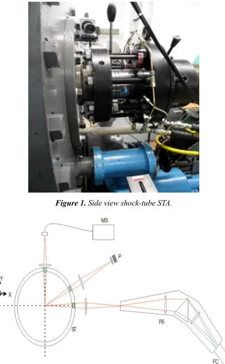
Figure 1. Side view shock-tube STA.
Figure 2. Experimental setup at shock-tube STA (ST=Shock-tube, MS=HR2000+ spectrometer, PS=Prism-spectrograph, P=Photodiode BPX65, FC= FAST-CAM camera.
measure a time integrated (20ms) broad band wavelength spectrum – spanned from 2000 Å to 9000 Å - for analysis of the emission process.
The recorded image spectra obtained from the combination of prism spectrograph and FAST-CAM-camera were then converted into wavelength spectra with the dispersion relation and corrected for the dark-signal. All the spectroscopic measurement equipment was triggered electronically by the control panel of the STA.
6. Calibration of the Experimental Setup
The dispersion-relation of the prism-spectrograph was obtained by inserting an Hg-Cd calibration lamp at that point inside the shock tube adapter ring were emission was imaged from (figures 1 and 2). With a standard tungsten ribbon lamp the black-body radiation signal at a current of 10 A which results in 2158 K was experimentally obtained in order to calculate the calibration curve. The calibration curve was used to determine the temperature from the emission spectra as described above.
7. Experimental Results
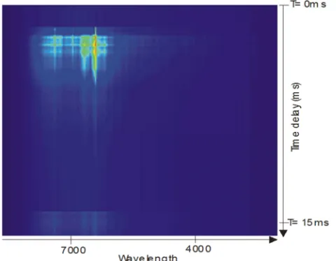
In figure 3 and figure 4 the experimental results at condition Mach 10 under gas condition nitrogen (Figure 3) and air condition (Figure 4) are illustrated.
Figure 3. Experimental time resolved emission spectra, nitrogen, M = 10, gate = 42µs, measurement window 15ms.
The images show the time evolution of spectral emission in the wavelength range between 3000 Å and 9000 Å during a time period of 15 ms. As it is obvious by comparing the figures the nitrogen condition shows to a lesser extent continuum radiation and pronounced atomic line emission. Besides this the air condition has a pronounced continuum emission with less atomic line emission. The line emission around 5000 Å is due to Sodium, Chromium, Lithium and Potassium as can be seen in figure 5, [15-16].
Figure 4. Experimental time resolved emission spectra, air M = 10, gate = 42µs, measurement window 15ms.
8. Evaluation of the Experimental
Results on Nitrogen
An example of spectra evaluation is shown in figure 5 (time delay ∆t =2.5 ms). The fitting of the Planck-function to the experimental measured spectrum at a fixed time delay including different parts of the radiation process (continuum- and atomic line radiation, Mach 10, gas nitrogen) can be seen.
Figure 5. Experimental result, nitrogen, Mach 10, ∆t = 2.5 ms, gate = 42µs.
green curve shows the fit of the Planck-function to the partial measurement data. It can be seen that neglecting atomic line emission a perfect match between experimental data and the fitting function can be obtained.
9. Time Resolved Temperature
Distribution
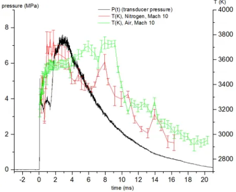
The evaluation of the experimental measured spectra gives the result of temperature distribution versus time at the given conditions as can be seen in figure 6.
Figure 6. Experimental result on pressure (black-curve) and on temperature distribution versus time (condition: nitrogen: red-curve, air: green-curve) at Mach=10, time frame ∆t = 15 ms.
The black curve in figure 6 gives the time resolved transducer pressure curve measured during the experiment. The red curve gives the temperature distribution versus time deduced from fitting the experimental measured emission spectra versus wavelength and time delay using nitrogen as a gaz. The green curve gives the temperature distribution versus time deduced from fitting the experimental measured emission spectra versus wavelength and time delay using air as a gaz. The graph shows that under air condition longer lasting, slightly higher temperatures are reached as it can also be deduced by comparing the intensity distribution from figures 3 and 4.
The comparison between predicted temperature distribution using traditional methods (from shock speed and pressure evolution in time) and results from emission spectroscopy shows less decay in time in the case using nitrogen as driver gas. In the case of air as driver gas we calculate an initial temperature of 3470 K and measure a initial temperature of 2450 K. The stagnation temperature in the case of air seems to increase during the first 2ms – and continues to rise thereafter, possibly due to the additional heat release at the gas interface (air/hydrogen).
The results obtained by measuring the light in the visible range emerging from the shock restricts possible evaluable temperatures down to 1500 K.
10. Conclusion
The data obtained from the spectroscopic investigations presented, demonstrate that the temporal evolution of the stagnation temperature can be measured with good accuracy and precision in both, nitrogen and air conditions. The emission spectroscopy technique is relatively easy to use, does not require a laser source and can replace the traditional shock-speed based post-experimental analysis tools.
The restriction of evaluable temperature values below 1500K can be circumvented by introducing a spectrometer working in the infrared region from 2.5 µm up to 10µm. Since the hydrodynamics of the shock tube is coming to be understood more fully, emission spectroscopy can be expected to provide quantitative (line broadening, temperature) data which have been unavailable. Of prime importance are Intensity of atomic and molecular line emission under known conditions. In this field, the shock tube appears to offer the investigation of temperature under controlled conditions.
Acknowledgements
We thank the Shock-tube Laboratory at ISL for the use of their equipment.
References
[1] Experimentelle Untersuchung der Umströmung von Gefechtsköpfen beim Eintritt in die Atmosphäre, ISL-RV 232/2010.
[2] Shock tunnels at ISL, ISL-U-PU 6106/2016.
[3] Zeitaufgelößte Strahldichtemessungen an stoßwellen-induzierten Blitzen in Argon, Luft und Xenon, ISL R 120 / 94. [4] M. R. E. Lamont, Y. Okawachi, and A. L. Gaeta, “Study about
lasers and optics,” Opt. Lett. 38, 3478 (2013).
[5] Fujii, T., Fukuchi, T., Laser Remote Sensing, CRC Press 2005. [6] Thorne, A., Litzen, U., Spectrophysics: Principles and
Applications, Germany, Springer, Berlin, Heidelberg, 1999. [7] D. Meiners, Spektroskopische Methoden zur Messung der
Temperatur in Plasmen mit Selbstabsorption, Bundesministerium für Bildung und Wissenschaft, Forschungsbericht K 72-22.
[8] Eichhorn, A., Werner, U., Zeitaufgelößte Temperaturmessung in Strömungen mit Rotationssymmetrie.
[9] S. W. Bowen, Spectroscopic and optical studies of a high pressure underexpanded jet, AIAA Plasmadynamics Conference, March 2-4, 1966.
[10] Buttsworth, D R., Jacobs, P. A., Total temperature measurement in a shock tunnel facility, 13th Australasian Fluid Mechanics Conference Monash University, Melbourne, Australia, 1998. [11] O’Byrne, S., Altenhofer, P., Time resolved temperature
[12] East, R., Perry, J., A short time response stagnation temperature probe, National Advisory Committee for Aeronautics, 1966.
[13] Widodo, A., Buttsworth, D., Stagnation temperature measurements in the USQ hypersonic wind tunnel, 17th Australasian Fluid Mechanics Conference Vol. 248, University of Auckland, 2010, pp. 840-844.
[14] Devia, D., M. Rodriguez-Restrepo, L. V., Methods employed in optical emission spectroscopy analysis, a review, Ingenieria y Ciencia-Universidad EAFIT, Vol. 11, No. 21, 2014, pp. 239-267.
[15] NIST, Atomic Spectra Database, Lines Data, MD 2015. [16] Hirata, R., Horagucci, T., Atomic Spectral Line List,