R E S E A R C H
Open Access
Robust surface normal estimation via
greedy sparse regression
Mingjing Zhang and Mark S. Drew
*Abstract
Photometric stereo (PST) is a widely used technique of estimating surface normals from an image set. However, it often produces inaccurate results for non-Lambertian surface reflectance. In this study, PST is reformulated as a sparse recovery problem where non-Lambertian errors are explicitly identified and corrected. We show that such a problem can be accurately solved via a greedy algorithm called orthogonal matching pursuit (OMP). The performance of OMP is evaluated on synthesized and real-world datasets: we found that the greedy algorithm is overall more robust to non-Lambertian errors than other state-of-the-art sparse approaches with little loss of efficiency. Along with providing an overview of current methods, novel contributions in this paper are as follows: we propose an alternative sparse formulation for PST; in previous PST studies (Wu et al., Robust photometric stereo via low-rank matrix completion and recovery, 2010), (S. Ikehata et al., Robust photometric stereo using sparse regression, 2012), the surface normal vector and the error vector are treated as two entities and are solved independently. In this study, we convert their
formulation into a new canonical form of the sparse recovery problem by combining the two vectors into one large vector in a new “stacked” formulation in this domain. This allows for a large repertoire of existing sparse recovery algorithms to be more straightforwardly applied to the PST problem. In our application of the OMP greedy algorithm, we show that greedy solvers can indeed be applied, with this study supplying the first of such attempt at employing greedy approaches to estimate surface normals within the framework of PST. We numerically compare the
performance of several normal vector recovery methods. Most notably, this is the first detailed test on complex images of the normal estimation accuracy of our previously proposed method, least median of squares (LMS).
Keywords: Photometric stereo, Robust, Surface normals, OMP
1 Introduction
Shading in 2D images provides a valuable visual cue for understanding the spatial structure of objects. Photomet-ric Stereo (PST) is a powerful technique that exploits shading information to directly estimate the 3D surface orientation, i.e. normal vectors. In the classical PST prob-lem, the input is a set ofnimages captured from a fixed viewpoint underndifferent calibrated lighting conditions; hence, there are n observations of luminance at each pixel location. Under the assumption of a Lambertian reflectance model, where the observed luminance is pro-portional to the cosine of the incident angle and remains constant regardless of the viewing angle, the relationship
*Correspondence: [email protected]
School of Computing Science, Simon Fraser University, Vancouver, BC V5A 1S6, Canada
betweennobservationsy∈Rnat each pixel and the col-lection ofnlighting directionsL∈Rn×3is formulated as a linear equation group with respect to the normal vector n∈R3, i.e.,
y=Ln. (1)
We emphasize that there are indeed such a set of n equation at each pixel. In PST, the linear system Eq. 1 is solved via ordinary least squares (LS). The advantage of PST over 3D laser scanning is that the former provides a very high resolution (depending on the actual resolution of the camera) and therefore can capture the fine details of the surface that may not show up in the scanned model. In addition, PST only requires a simple and inexpensive hardware setup whereas 3D scanning devices are usually costly and less portable. Innovative recent work [3, 4] can reduce PST to a single-shot scenario in a different setup
with spectral multiplexing and more than three colour channels or polarized illumination.
Although the classical PST method almost always guar-antees a visually plausible normal map, it in fact suffers from a serious accuracy problem: the simple Lambertian reflectance model adopted in PST does not strictly apply to most real-world textures, which exhibit specular reflec-tion properties to various degrees. Even if the surface is indeed approximately Lambertian, other non-Lambertian errors can be introduced by the interaction of the light and the objects’ geometry, resulting in cast shadows, includ-ing self-shadowinclud-ing, as well as interreflections. Attached shadows are also outside the simple shading model. Such non-Lambertian observations, regarded as “outliers” in a Lambertian-based linear model, may severely reduce the accuracy of LS results. Hence, a PST method that is robust to such non-Lambertian effects is needed in order to generate a high-quality normal map.
Many improved PST methods have been proposed since the original PST in an attempt to minimize the effect of non-Lambertian components. These methods either adopt a more sophisticated reflectance model to accommodate non-Lambertian observations as “inliers” (e.g. [5–7]) or rather keep the Lambertian model but use robust statistical methods to rule out or reduce the effect of non-Lambertian outliers (e.g. [8–10]). A typi-cal example of the second category is the least median of squares (LMS) approach used in our previous study
[11] (and see [10, 12]), in which the observations out-side a certain confidence band are deemed to be outliers. In this study, we again adopt the Lambertian model, but solve for the normal vectors via a sparse represen-tation framework that estimates both the normals and non-Lambertian errors at the same time. This sparse method is more closely related to the statistical-based methods.
1.1 Sparse representation and recovery
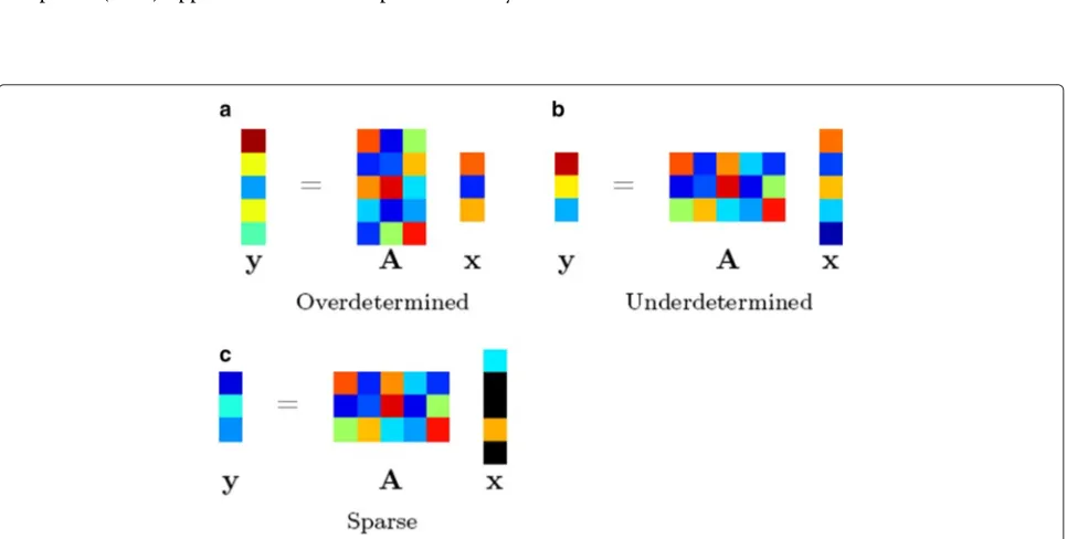
It is well understood that ordinary LS fails to unambigu-ously reconstruct a signal that is passed through an under-determined linear system, where the number of unknown variables exceeds that of linear equations (Fig. 1b). How-ever, it has been shown that if the signal to be recov-ered is sparse—having a considerable number of zero or nearly zero entries (Fig. 1c)—then an accurate reconstruc-tion of the signal is still possible via a sparse recovery scheme [13].
The canonical form of a sparse recovery problem can be stated as follows: given an underdetermined linear model y = Ax, where A ∈ Rn×p is the so-called dictionary matrix (n < p), and y ∈ Rn×1is the vector consisting ofnscalar observations, find the unknown sparse signal x∈Rp×1such that
min
x x0 s.t. y=Ax, (2)
where ·0 represents 0 pseudo-norm, the number of
non-zero entries.
Equation 2 is generally a non-deterministic polynomial-time (NP)-hard combinatorial problem [14]. In practice, it is more feasible to solve a relaxed form. We will briefly dis-cuss various alternative formulations and corresponding solvers in Section 2.2.
1.2 Photometric stereo and sparse recovery
PST is often formulated as an overdetermined regres-sion problem. The classical PST adopts three lights (hence three observations of luminance at each pixel location) [15] to solve for the 3D normal vectors. Later methods use more lights ranging from four to hundreds [6, 10, 16, 17]. Recently, a few attempts have been made to represent PST as an underdetermined system; firstly, in the case of calibrated lighting directions [1, 2], as addressed here, as well as for the alternative case of unknown lighting conditions [18, 19], not studied in this report. Reconfigur-ing PST as an underdetermined system means explicitly modelling the non-Lambertian error for each observa-tion as addiobserva-tional unknowns. Suppose there arenlights (hencenequations for each pixel): the per-pixel number of unknowns would ben+3 (three normal vector com-ponents and n non-Lambertian errors). As was already pointed out, such a system cannot be unambiguously solved through ordinary LS. Fortunately, if we make an assumption that the majority of luminance observations are approximately Lambertian, then the error vector is essentially a sparse vector with a large number of zero or approximately zero entries. Now that we have a sparse representation of the PST problem, we can solve it using a sparse recovery algorithm.
It has been shown by Wu et al. [1] and Ikehata et al. [2] that sparse PST behaves significantly more robustly than the classical PST method. However, the accuracy is con-tingent on the solver. At present, the most accurate solver for the sparse formulation is sparse Bayesian learning (SBL) as tested by Ikehata et al. in [2]. In the current study, we employ a modified form of the sparse representation given in [2], but solve it via a different approach—greedy sparse recovery algorithms.
1.3 Novel contributions
The main contributions of the current study are threefold:
1. We propose an alternative sparse formulation for PST (Eqs. 10 and 11). In previous PST studies [1, 2], the surface normal vector and the error vector are treated as two entities and are solved independently. In this study, we convert their formulation into a new canonical form of the sparse recovery problem by combining the two vectors into one large vector. Although such a “stacked” formulation is not novel
(e.g. [20]), it is used in the context of surface normal estimation for the first time. The advantage of this formulation is that it allows for a large repertoire of existing sparse recovery algorithms to be more straightforwardly applied to the PST problem. 2. We apply a greedy algorithm called orthogonal
matching pursuit (OMP) [21–23], from information theory, to solve the PST problem. It has been previously demonstrated in [1, 2] that PST can be solved by several sparse recovery algorithms that fall into different categories, including augmented Lagrangian rank-minimization [1],1optimization approaches and probability-based methods [2]. However, the possibility of applying greedy solvers, an important category of sparse recovery algorithms, to the PST problem has never been explored. To the best of our knowledge, this study is the first of such attempt at employing greedy approaches to estimate surface normals within the framework of PST. 3. We numerically compare the performance of several
normal vector recovery methods. Most notably, it is the first time that the normal estimation accuracy of our previously proposed method—LMS—has been tested and quantitatively demonstrated on complex models.
1.4 Overview
This paper is organized as follows: Section 2 provides a short survey on recent robust PST and sparse recovery methods. In Section 3, we provide a detailed description of our sparse formulation and the OMP algorithm. Exper-imental results and discussions are presented in Section 4, followed by several possible future research directions discussed in Section 5.
2 Related work
2.1 Robust photometric stereo
This section presents a brief overview of current PST methods. Since the original non-robust Lambertian-based PST [15], many methods have been proposed in an attempt to address non-Lambertian effects such as spec-ularities and shadows. These approaches usually adopt a robust statistical method and/or an improved non-Lambertian reflectance model.
2.1.1 Statistics-based methods
to highlights and shadows, are simply discarded. Another four-light method [26] explicitly included ambient illumi-nation and surface integrability and adopted an iterative strategy, using current surface estimates to accept or reject each additional light based on a threshold indicating a shadowed value. The problem with these methods is that they rely on throwing away a small number of outlier observation values, whereas our robust sparse methods in the current study reaches the solution based on all obser-vations, by correcting the non-Lambertian error of the outlier observations.
Willems et al. [27] used an iterative method to esti-mate normals. Initially, the pixel values within a certain range (10–240 out of 255) were used to estimate an ini-tial normal map. In each of the following iterations, error residuals of normals for all lighting directions are com-puted and the normals are updated based only on those directions with small residuals. Sun et al. [28] showed that at least six light sources are needed to guarantee that every location on the surface is illuminated by at least three lights. They proposed a decision algorithm to discard only doubtful pixels, rather than throwing away all pixel val-ues that lie outside a certain range. However, the validity of their method is based on the assumption that out of the six values for each pixel, there is at most one highlight pixels and two shadowed pixels. Mallick et al. [29] intro-duced a method based on colour space transformation to separate specular and diffuse components. Holroyd et al. [30] exploited the symmetries in the 2D slices of bidirec-tional reflectance distribution function (BRDF) obtained at each pixel to recover surface normal and tangent vec-tors. Both [29] and [30] can be applied to a great variety of surface reflectance, but they do not provide enough focus on the robustness against shadow pixels. Julià et al. [31] utilized a factorization technique to decompose the lumi-nance matrix into surface and light source matrices. They consider the shadow and highlight pixels as missing data, with the objective of reducing the influence of these pixels on the final result.
Some recent studies utilize probability models as a mechanism to incorporate the handling of shadows and highlights into the PST formulation. Tang et al. [32] model normal orientations and discontinuities with two coupled Markov random fields (MRF). They proposed a tenso-rial belief propagation method to solve themaximum a posteriori(MAP) problem in the Markov network. Chan-draker et al. [33] formulate PST as a shadow labelling problem where the labels of each pixel’s neighbours are taken into consideration, enforcing the smoothness of the shadowed region, and approximate the solution via a fast iterative graph-cut method. Another study [8] employs a maximum likelihood (ML) imaging model for PST. In this method, an inlier map modelled via MRF is included in the ML model. However, the initial values of the inlier
map would directly influence the final result, whereas our sparse method does not depend on the choice of any prior. A few other studies employ random-sampling-based methods. Using three-light datasets, Mukaigawa et al. [34] adopt a random sample consensus (RANSAC)-based approach to iteratively select random groups of pixels from different regions of the image, and the sampled group whose pixels are all taken from diffuse regions are used to calculate the coefficients in the linear equation. RANSAC is also used in a multiview context [9] as a robust fitting approach to select the points on a certain 3D curve. Drew et al. [10, 12] and Zhang and Drew [11] employ a LMS method. Instead of taking samples from different regions on the image, they use a denser image set (50 lights) and sample only from the observations at each pixel location. Non-Lambertian observations are rejected as outliers and excluded from the following LS step. Based on [33], Miyazaki et al. [35] used a median filtering approach similar to LMS but also considering neighbouring pixels. Instead of taking random samples, they simply compare all the three combinations of obser-vations, which is feasible for the small number of lights used in their study. Although guaranteeing a high statisti-cal robustness, these methods are computationally heavy since they usually rely on a large number of samples to take effect.
2.1.2 Non-Lambertian reflectance modelling
Instead of statistically rejecting non-Lambertian effects as outliers, another way to minimize their negative influ-ence on surface normal recovery is to incorporate a more sophisticated reflectance model to directly account for the non-Lambertian components.
Tagare and de Figueiredo [36] constructed an m-lobed reflectance map model to approximate diffuse non-Lambertian surface-light interactions. In [25], a Torrance-Sparrow model is employed to estimate the roughness of the surface that is divided into different areas. Similarly, Nayar et al. [37] adopt a Torrance-Sparrow and Beckmann-Spizzichino hybrid reflectance model. Georghiades [38] applied Torrance-Sparrow model to handle the uncalibrated photometric stereo problem. Other mathematical models to encode surface reflectance include polynomial texture mapping (PTM) [39] and spherical harmonics (SH) [40]. Drew et al. [10] proposed a radial basis function (RBF) interpolation to handle the rendering of specularities and shadows.
of other objects with similar reflectance as the reference object can simply be inferred from the look-up table. This method, however, only applies to isotropic materi-als. Hertzmann and Seitz [5] later revisited the idea of including reference material. By adopting an orientation-consistency cue assumption that two points on the surface with the same orientation have the same observed light intensity, they effectively cast PST as a stereoptic corre-spondence problem. This approach is capable of handling a wider range of anisotropic materials with a small num-ber of reference objects, usually one or two. Similar to [5], an appearance-clustering method proposed by Koppal and Narasimhan [42], also adopting the orientation con-sistency cue, focuses on finding iso-normals across frames in a captured image sequence, and a classical PST approach may be applied later to obtain the accurate value of the surface normals. Although their method does not rely on the presence of a reference object, it does require the image sequence to be densely captured on a continuous path.
Recent studies attempt to solve a more complicated problem where neither shape nor material informa-tion of the object surface is available. Goldman et al. [43] employed an objective function that contains terms for both shape and material and proposed an iterative approach where the reflectance and shape are alternately optimized. The estimation of the material is an insep-arable part of the reconstruction process so an explicit reference object is no longer needed. Alldrin et al. [6] also adopt a similar iterative approach that updates shapes and materials alternately. Their formulation is non-parametric and data-driven, and as such is capable of capturing an even wider range of reflectance materials. Ackermann et al. [7] proposed an example-based multi-view PST method which uses the captured object’s own geometry as reference.
Yang et al. [44] include a dichromatic reflection model into PST for both estimating surface normals as well as separating the diffuse and specular components, based on a surface chromaticity invariant. Their method is able to reduce the specular effect even when the specular-free observability assumption (that is, each pixel is diffuse in at least one input image) is violated. However, this method does not address shadows and fails on surfaces that mix their own colours into the reflected highlights, such as metallic materials. Moreover, their method also requires knowledge of the lighting chromaticity—they suggest a simple white-patch estimator—whereas in our method, we have no such requirement. Kherada et al. [45] pro-posed a component-based mapping (CBM) method. They decompose the captured images into direct components (single bounce of light from a surface) and global compo-nents (illumination onto a point that is interreflected from all other points in the scene). They then model matte,
shadow and specularity separately within each compo-nent. This method depends on a training phase, requires accurate disambiguation of direct and global contribu-tions and has a high computational load. Shi et al. [46] introduced a bi-polynomial representation to model the low-frequency component of reflectance and used only the low-frequency information to recover shape and esti-mate reflectance.
The problem with these methods is that they usually do not work well against non-Lambertian effects that are not accounted for by the surface reflectance alone, such as cast shadows. In our current sparse method, we make no assumption of the surface reflectance property and treat all non-Lambertian effects (specularity and shadow) equally.
2.1.3 Sparse formulation
Recently, a few studies began to adopt sparse representa-tion into PST. Wu et al. [1] model the matrix of all lumi-nance observations as a linear combination of Lambertian and Lambertian components and represent the non-Lambertian error as an additive sparse noise vector. Under the assumption that most pixel observations approxi-mately follow the Lambertian reflectance model, they obtain the solution by finding a sparse vector such that the rank of the Lambertian component matrix is minimized. The formulation is known as robust principal component analysis (R-PCA) in the field of sparse recovery. Specifi-cally, they adopted a fast and scalable algorithm suitable for handling a large amount of data points, i.e. the aug-mented Lagrange multiplier method [47]. However, this method requires a shadow mask to be specified explicitly. Later, Ikehata et al. [2] reconsider PST as a pure sparse regression problem and aim to minimize the number of entries (i.e. the0pseudo norm) in the error matrix. They
also add an2relaxation term to account for cases when
the sparse assumption is violated. In order to avoid the difficult combinatorial problem involved in the minimiza-tion of0norm, they introduced two possible algorithms.
One is to relax the 0 pseudo norm into 1 norm, as
a matte image with specularity and shadows attenuated, whereas the present work is aimed at accurate normal-vector recovery. Whereas our use of OMP uses a greedy algorithm where each component is picked one at a time, in contrast, the ADMM approach adjusts all the compo-nents in each iteration. The present study is the first to use greedy approaches to surface normal estimation within a PST framework.
Sparse methods have also found their use in uncali-brated PST, where the lighting directions are not known (but note that in this study we do assume known lighting directions so that these works are somewhat peripheral). Favaro et al. [18] incorporate the rank-minimization algo-rithm proposed in [1] into the uncalibrated PST problem as a pre-processing step to remove shadow and specular-ity effects. Argyriou et al. [19] recently also adopt a sparse representation framework to decide the weights for find-ing the best illuminants to use, again with the lightfind-ing directions unknown.
2.2 Sparse recovery methods
As was pointed out in Section 1.1, the canonical form of the sparse recovery problem (Eq. 2) is NP-hard [14] and cannot be solved efficiently as-is. In this section, we sum-marize alternative formulations to Eq. 2 and several types of solvers.
The first type of approach is convex1relaxation. It has
been shown that for a dictionary matrixAthat satisfies a certain restriction, Eq. 2 is likely to be equivalent to an1
minimization problem [13, 48]:
min
x x1 s.t. y=Ax, (3)
which can be solved via convex optimization techniques such as interior-point (IP) methods [52], gradient projec-tion [53], IRL1 [49] and so forth.
Alternatively, sparse recovery can be achieved via greedy algorithms. The basic idea of such an algorithm is employing an iterative method to find the collection of non-zero entries, orsupport, of the signalx, and then recoverxvia LS using only the observations in the sup-port.
One of the most notable greedy algorithms is OMP [21–23], an improvement over the simple matching pur-suit (MP) algorithm [54]. In OMP, a column aj in Ais
iteratively chosen such thataj is most greatly correlated
with the current residualr. Then,ris updated by taking into consideration the contribution ofaj. The algorithm
is terminated as a fixed number of non-zero entries are recovered or other stopping criteria are met. Then, a sim-ple LS is performed only on a submatrix ofAconsisting of the columns chosen by OMP, and the regressed result will be assigned only to the signal entries corresponding to the selected columns. The columns that are not selected by OMP, on the other hand, will not be used in the final LS
step, and their corresponding signal entries are simply set to zero.
In fact, OMP approximately solves the following k -sparse recovery problem:
min
x y−Ax2 s.t. x0≤k. (4)
Many state-of-the-art greedy algorithms nowadays are based on OMP. Examples include regularized OMP (ROMP) [55, 56], stagewise OMP (StOMP) [57], compres-sive sampling matching pursuit (CoSaMP) [58], probabil-ity OMP (PrOMP) [59], look ahead OMP [60], OMP with replacement (OMPR) [61], A* OMP [62] etc.
Another type of solvers employ a thresholding step to iteratively refine the recovered support, i.e. the selec-tion/rejection of an entry at each step, is decided by whether the value of a certain function dependent on this entry falls below a given threshold. Algorithms in this category include iterative hard thresholding (IHT) [63], subspace pursuit (SP) [64], approximate message passing (AMP) [65], two-stage thresholding (TST) [66], algebraic pursuit (ALPS) [67] etc.
The fourth category is probability-based algorithms. These methods assume the signal to be recovered follows a specific probability distribution and solve the sparse recovery problem with statistical methods such as ML or MAP estimation. SBL [50] is one of the major algo-rithms in this category and has already been applied in the context of PST [2].
3 Sparse regression
3.1 Sparse formulation for photometric stereo
In this section, we explore the possibility of formulating and solving PST as a sparse regression problem. Since only the normal recovery is studied in this paper, we omit the albedo α from all equations in this and the follow-ing sections for simplicity and always usento represent the unnormalised surface normal vector unless otherwise specified.
Here, we assume a Lambertian reflectance model with an additional term e ∈ R to account for the non-Lambertian error. Hence, the observed luminance ycan be expressed as:
y=l·n+e, (5)
wherel∈R3andn∈R3represent the lighting direction and surface normal, respectively. For each pixel, we haven observationsy =(y1,y2,. . .yn)T ∈Rn. Now, let us write
Eq. 5 in vector form
y=Ln+e, (6)
where L = (l1,l2,. . .ln)T ∈ Rn×3 and e =
(e1,e2,. . .en)T ∈Rn.
n), is effectively an underdetermined problem and as such cannot be solved unambiguously. However, if the errore is a sparse matrix, i.e. most or at least a great percentage of its elements are zero, then it is still possible to recover eexactly or almost exactly by solving the following sparse regression problem:
min
n,e e0 s.t. y=Ln+e. (7)
In Eq. 7, ·0 represents the 0 pseudo-norm or the
number of non-zero elements in e. This formulation, however, has two major issues: (1) it is an NP-hard com-binatorial problem and (2) real-world scenes may contain a large variety of materials that are only poorly approx-imated by the Lambertian reflectance model. For those materials, it is very likely thateis not strictly sparse. Thus, the equality constraint is very hard to be satisfied. Instead, it is more realistic to use an inequality constraint with a user-defined error tolerance
min
n,e e0 s.t. y−Ln−e2≤. (8)
Alternatively, if we care more about how much the reconstructed luminance approximates real observation rather than the sparsity ofe, then it would be more natural to reformulate Eq. 8 as
min
n,e y−Ln−e2 s.t. e0≤s, (9)
where the scalar sis the sparsity of vector e. To further simplify Eq. 9, we propose mergingnandeinto one large vector and treating them as one entity, i.e.
y=Ln+e =Ln+Ie
=(L,I)
n e
=Ax,
(10)
whereI∈Rn×nis ann×nidentity matrix,A=(L,I) ∈ Rn×(n+3) is a new merged dictionary matrix and x =
(nT,eT)T ∈ R(n+3)×1 is the combined vector of all the
unknown variables. Hence, Eq. 9 can be rewritten as
min
n,e y−Ax2 s.t. x0≤s. (11)
The stacked formulation was inspired by the work of Wright et al. [20, Eq. 20]. However, in [20], both the signal and the noise are assumed sparse, whereas in our case, the signal (normal vector) has only three components and is not at all sparse.
By formulating our problem in the form of Eq. 11, we can now take advantage of existing algorithms to effi-ciently achieve an accurate solution. One such solver is a greedy algorithm known as OMP [21–23], which is known for its high accuracy and low time-complexity. We will describe this algorithm in Section 3.2 in detail.
Previously, Ikehata et al. [2] proposed a different for-mulation to Eq. 11. They expressed the PST problem in a so-called Lagrangian form, i.e.
min
n,e y−Ln−e
2
2+λe1 (12)
and applied two solving algorithms: IRL1 minimization and SBL. They showed that SBL provides a more accurate estimation but is more computationally expensive. Later, in Section 4, we will show that our OMP solver produces a more accurate result than SBL with comparable efficiency to IRL1.
3.2 Orthogonal matching pursuit
Sparse recovery problems like Eq. 11 can be solved via many different methods (see Section 2.2 for a brief overview). Here, we choose to apply the classical greedy OMP to our surface normal recovery problem. Given the
Fig. 2Visualization of all observations of one pixel from datasetCaesar.aThe pixel studied is marked withblue crossesat the same location (X=90,Y=39) on all images numbered from 1 to 50.bLuminance observations arranged by the image index 1 to 50.cLuminance observations sorted by incident angle.Blue dotted lineshows the actual 50 observations;red circled lineshows the approximated luminance using least squares;
Fig. 3Outliers identified by orthogonal matching pursuit.aOutliers with great non-Lambertian error (red circles) detected in iterations 4–10. bOutliers with medium to great error (red circles) detected in iterations 4–18.cAll outliers (red circles) detected as of iteration 28.Blue dotted lines
show actual luminance observations in all three plots
linear model in Eq. 10, the basic idea of OMP is to itera-tively select columns of the dictionary matrixAthat are most closely correlated with the current residuals, then project the observationyto the linear subspace spanned by the columns selected until the current iteration. We denote each column ofAasAj.
Letibe the current number of iterations andri andci
the residuals and the subset of selected columns inAat theith iteration, respectively. LetA(ci)andx(ci)represent
the columns indexed byciinAand the entries indexed by ciin the signalxto be recovered, respectively. The OMP
algorithm [23], as we here apply to our PST problem, can be summarized as follows:
AlgorithmOrthogonal matching pursuit
1. Normalise each column of the dictionary matrixA and denote the resulting matrix asA, i.e.Aj2=1 forj=1, 2,. . .,p. Initialize the iteration counter i=1, residualr0=yandc0=∅.
2. Find a columnAt(t∈ {1, 2,. . .,p} −ci−1) that is most closely correlated with the current residual. Equivalently, solve the following maximization problem:
t=argmax
j A
T
j ri−1 (13)
3. Addt to the selected set of columns, i.e. update ci=ci−1∪t, and useA(ci)as the current selected subset ofA.
4. Project the observationyonto the linear space spanned byA(ci). The projection matrix is calculated as follows:
P=A(ci)(A(ci)TA(ci))(−1)A(ci)T. (14)
5. Update the residuals with respect to the new projected observation
ri=y−Py. (15)
6. Incrementi by 1. Ifi>n/2+3(= 28 for our typical datasets of 50 images), then proceed to step 7, otherwise go back to step 2.
7. Solve only for the entries indexed byciin signalx using the original,unnormaliseddesign matrixA, and simply set the rest of the entries to 0, i.e.
x(ci)=A(ci)†y (16)
and
xj=0 for each j∈/ci. (17)
8. Take the first three entries inxas the solutions for thex, y and z component of the normal vector, respectively,
n=(x1,x2,x3). (18)
Fig. 4Matte component recovered by orthogonal matching pursuit.
In our formulation Eq. 10, we merge the normal and the errors into a large vector, so the components of the two vectors are treated equally by OMP. In each iteration, which column in the dictionary matrix is to be chosen purely depends on its correlation with the current resid-uals. Thus, there is no strict mathematical guarantee that the normal vector components will be selected in the first siterations. Indeed, this failure could happen if the non-Lambertian error vector accounts for most of the observa-tions. However, since the observed luminance is usually a function of the surface normal, it is expected that the nor-mal vector components are more closely correlated to the
observations than the sporadic non-Lambertian errors. In our experiments, all normal vector components are usu-ally selected within the first few iterations (<10). On the other hand, if one or two components of the surface nor-mal are rather snor-mall, then they might not be selected by our algorithm. However, since they are very close to zero anyway, simply treating them as zero would not negatively impact the accuracy of our estimation.
One of the biggest advantages of OMP is its low com-putational cost and straightforward implementation. We have found that it is significantly faster than LMS as well as other state-of-the-art robust regression methods that
have been applied in the context of PST (see Section 4.3 and Fig. 21 for more details). Note that for our particu-lar choice of the design matrixA, the correlation between any column in the identity matrix and the residualrcan be simply represented by one element in r. Therefore, the inner product in Eq. 13 may be reduced to finding the maximum entry inr. This observation allows for an even more efficient implementation. In this work, how-ever, we still implement OMP according to Eq. 13 for generality.
3.2.1 Normalization and orthogonality
As a requirement of the standard OMP algorithm, we used the column normalised version of the design matrix A in the column selecting process. After normalization, the
first three columns inAno longer hold the correct value of lighting vector components. In other words, it appears that the lighting directions are modified by normaliza-tion. However, this observation does not negatively affect our results. In step 2 of OMP, the column most correlated with the current residual vector is selected. Normalization only makes sure one column does not have a numerical advantage over another simply because it has a greater L2 norm. Therefore, normalization does not interferes with the selection of the outliers. On the contrary, it enforces the correctness of selection. It is also important to note that after the outliers are selected, we use the original unnormalised dictionary matrixA, instead ofA, to make sure that the normal vector are recovered on the actual lighting directions.
Another issue worth noting is the orthogonality of the dictionary matrixA. It has been shown that ifAsatisfies a restricted isometry property (RIP), then the exact recov-ery of signalxmay be possible [68, 69]. Essentially, RIP specifies a near-orthonormal condition forA. Although our dictionary matrixAunfortunately does not obey the RIP property in its general form, we still argue that this matrix is near-orthogonal: with our uniform light distri-bution, the first three columns are indeed near-orthogonal (the dot products between column 1–2, 1–3 and 2–3 are 8.85 × 10⁻⁸,−1.04 × 0−6and−5.17× 10⁻⁷, respec-tively). The rest ofAis a large identity matrixI, which itself is orthonormal. Also, due to the large number of zeros in I, the dot product of any of the first three columns and any column inIis a rather small number (10−3−10−2scale on
average). Thus, although it is yet to be strictly proven, we speculate that the dictionary matrixAin near-orthogonal enough for our purpose of recovering the three com-ponents of normal out of the 53-element signal. As our results show, OMP indeed achieves highly precise recov-ery of surface normal for most of the pixel locations (see Section 4). We also show that even with a very biased lighting distribution (such that the orthogonality of the first three column are greatly reduced), OMP still provides an accepted recovery with higher accuracy than other sparse methods (see Section 4.2.4).
3.2.2 Stopping criterion
For simplicity, here we set the stopping criterion as a fixed number (s) of iterations. We make a conservative
assumption that 50 % of the observed pixels are polluted by non-Lambertian noise. Thus, for our typical datasets ofn = 50 images and normal vectors with three compo-nents, the stopping criterion isi>s=n/2+3=28. This criterion ensures that there is always a moderate number of observations (25) available for regression.
An alternative choice of stopping criterion is based on the residual, i.e. |r| < threshold. It has been proved that in the matching pursuit and its orthogonal version, OMP, are guaranteed to converge [21, 54]. Thus, such a stopping criterion is theoretically viable. Indeed, we have validated that in our OMP-based method, the residual converges on all pixels used in our datasets. However, we have also noticed in our tests that setting a hard thresh-old for all pixels results in a slightly decreased accuracy
than using the sparsity-based criterion (results not shown). Therefore, in the current study, we will continue using the sparsity-based criterion, i.e.i>=28.
3.3 Visual demonstration
In this section, we demonstrate how OMP enforces robustness onto the normal recovery process by using a simple example. Particularly, we use a synthesized datasetCaesar (see Section 4.1.1 for more information) and study all the 50 observations of one pixel (marked by blue crosses in Fig. 2a) at location (X = 90,Y = 39) where the ground truth normal vector is ngt =
(−0.0780, 0.1828, 0.9801). The luminance profile of these observations, sorted by incident light angle, are shown in Fig. 2c (blue dotted line), along with the actual matte
model curve (black solid line), i.e. the theoretical values of luminance, if the surface is purely Lambertian. It is obvious from Fig. 2c that due to the existence of specular reflection, a good percentage of observations (especially when the incident angle is small) deviate from the values predicted by a matte model.
The naive LS regression, when applied to this pixel, attempts to approximate the values of all observations without taking the actual matte model into consideration (Fig. 2c, red line marked with circles). Naturally, the LS result nLS = (−0.1578, 0.4852, 0.8600) deviates greatly
from the ground truth(−0.0780, 0.1828, 0.9801).
On the other hand, OMP first attempts to identify s entries, one in each iteration, from the stacked signalx= (x1,x2,. . .xn+3)T ∈ Rn+3 (see Eq. 10). Usually, theses
entries include three components for normal vectors (x1, x2, x3) and (s − 3) components from the remaining n
entries (x4,x5,. . .,xn+3) that correspond to error values.
When the OMP algorithm as described in Section 3.2 is applied to this pixel, it behaves as follows:
Iterations 1–3: The entries that correspond to normal vectors,x3,x2andx1, are selected in the order listed. This
is not a coincidence since the first three columns of the
dictionary matrixAare overall more strongly correlated to the observations than any of the rest of the columns that correspond to noise values. Also, we noticed that these entries are in fact selected in order of the abso-lute value of their corresponding normal components. For instance, the third component of the ground truth nor-mal (−0.0780, 0.1828, 0.9801) is greater than the other two components. Therefore,x3gets selected in the first
iteration.
Iterations 4–10: Entries x26, x15, x32, x9, x37, x21 and x20are selected sequentially. These entries correspond to
non-Lambertian errors at observation #23, #12, . . . #17, respectively (marked with red circles in Fig. 3a). Note that the indices of observations mentioned here (23, 12, . . . ) are equal to the entry indices found (26, 15, . . . ) minus 3, since the first three elements in x do not represent errors. We notice that the corresponding observations of these selected entries all have very high error val-ues. As in iterations 1–3, these error entries are also selected in order of their absolute value. For instance, observation #23 (incident angle ≈ 32°) has the great-est non-Lambertian error; therefore, its corresponding error entry x26 is selected in iteration 4, before other
entries.
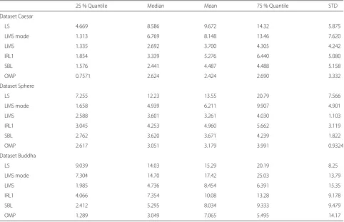
Table 1Statistics for the angular error between the normal maps recovered for various methods and the ground truth, for three synthesized datasets. All numbers are shown in degrees
25 % Quantile Median Mean 75 % Quantile STD
Dataset Caesar
LS 4.669 8.586 9.672 14.32 5.875
LMS mode 1.313 6.769 8.148 13.46 7.620
LMS 1.335 2.692 3.700 4.305 4.242
IRL1 1.854 3.339 5.276 6.440 5.080
SBL 1.576 2.441 4.487 4.488 5.158
OMP 0.7571 2.624 2.424 2.690 3.332
Dataset Sphere
LS 7.255 12.23 13.55 20.79 7.566
LMS mode 1.658 4.939 6.211 9.907 4.901
LMS 2.588 3.601 3.261 4.030 1.103
IRL1 3.045 4.253 4.960 5.662 3.119
SBL 2.762 3.620 3.671 4.239 1.822
OMP 2.617 3.051 3.179 3.991 0.9324
Dataset Buddha
LS 9.039 14.03 15.29 20.19 8.25
LMS mode 7.304 14.70 17.42 25.03 13.79
LMS 1.985 4.736 8.454 6.391 15.35
IRL1 4.066 7.354 10.08 13.28 9.178
SBL 2.412 5.295 8.034 9.333 9.479
Iterations 11–18: Another eight entries x4, x10, x42, x8, x14, x51, x48 and x5 are selected sequentially. Their
corresponding observations have medium error values (Fig. 3b).
Iterations 19–28: Select the rest of the error entriesx43, x27,x50,x31,x16,x7,x13,x6,x53andx25. The
correspond-ing observations have small error values (Fig. 3c).
Through the 28 iterations above, we have obtained 28 indices; 3 of them correspond to the normal-vector com-ponents and the remaining 25 represent the observations that have significant non-Lambertian effect, i.e. non-zero values in signalxin the sparse regression problem y =
Ax (Eq. 10). Suppose the indices of 25 selected non-Lambertian outliers are collectively represented ascout⊂ {1, 2,. . ., 50}, we can obtain the normal vectornand an error vectoreby solving the following equation (which is essentially the same as 16):
y=(L,I(cout))
n e(cout)
. (19)
For our sample pixel, the above equation givesnOMP =
(−0.0877, 0.2282, 0.9697), which well approximates the ground truth ngt = (−0.078, 0.1828, 0.9801) compared
to the naive LS result nLS = (−0.1578, 0.4852, 0.8600).
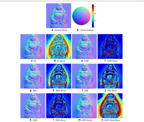
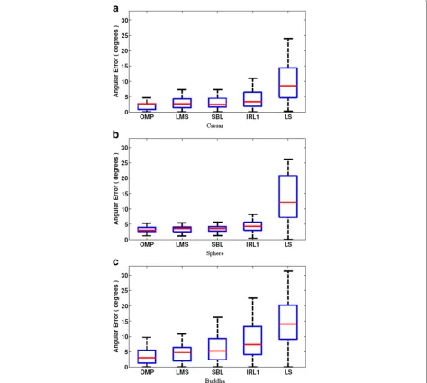
Fig. 9Angular error of normal maps recovered using various methods (a–c).Red horizontal linesindicate medians. Upper and lower border of the
Fig. 10Three-dimensional surfaces reconstructed from normal maps.bDepth map recovered with the ground truth normal map.a,d,e,c,fDepth maps recovered using LS, IRL1, OMP, LMS and SBL, respectively
Additionally, we can directly recover the matte compo-nents by subtracting the error vector efrom the actual luminance observationy. Note that the matte components obtained this way (Fig. 4, red solid line) almost coincide with the ground truth matte model, exhibiting a high degree of robustness.
4 Results and discussion
In this chapter, we present our experimental results and observations on synthesized and real datasets. All experi-ments were carried out on a Dell Optiplex 755 computer
equipped with an Intel Core Duo E6550 CPU and 4 GB RAM, running Windows 7 Enterprise 64 bit. All algo-rithms were implemented in MATLAB R2014a 64 bit.
4.1 Normal map recovery
We first examine the angular error of normal maps recovered by different methods on both synthesized and real datasets. For synthesized datasets, we quanti-tatively inspect the difference between the ground truth normal map and the recovered normal maps. For real datasets without a ground truth map, on the other hand,
the recovered normal maps are examined visually and qualitatively.
4.1.1 Synthesized datasets
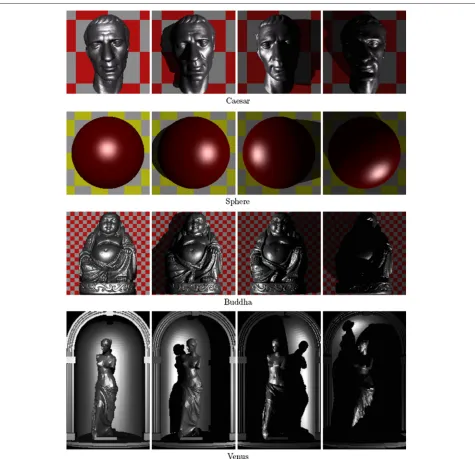
Four 3D objects are used for our synthesized datasets in this study: Sphere, Caesar, Buddha and Venus. All 3D models are either created programmatically as geo-metrical primitives (Sphere) or downloaded from the AIM@SHAPE Shape Repository (Caesar, Buddha) [70] and the INRIA Gamma research database (Venus) [71]. For each object, 50 images are rendered under various lighting directions using raytracing software (POV-Ray 3.6) at a resolution of 200×200 (except forVenus, whose resolution is 150×250). Global illumination is enabled to ensure a highly photorealistic appearance. All scenes fea-ture significant specularity and large areas of cast shadow. Caesar,Buddha and Venusare rendered with the spec-ular highlight shading model provided by POV-Ray (a modified version of the Phong model) [72], and Sphere is rendered with a pure Phong model. A checkered plane is intentionally included in the rendered scene as back-ground to (1) allow for the cast shadow to appear and (2) add further challenges to the algorithms since it intro-duces local fluctuation in luminance while the surface nor-mals remain constant. Sample images for these datasets are shown in Fig. 5.
For each image set, the normal map is estimated using the OMP method [21–23] as proposed in this study. For comparison, we show the results for two other state-of-the-art sparse recovery methods—IRL1 and SBL [2].
Another two of our previously proposed outlier detection-based methods, LMS [10] and LMS mode finder [11], are also applied and compared. Then, the angular error between the normal map recovered using each method and the ground truth is quantitatively measured. Note that only results forCaesar,SphereandBuddhaare shown in this section. The fourth datasetVenusis reserved for later in Section 4.2.2 as a failure case.
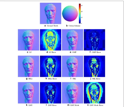
We found these methods exhibit similar relative perfor-mance to each other on all the three datasets tested in this section—Sphere,CaesarandBuddha. InCaesar, the nor-mal maps recovered using OMP (Fig. 6e) have a higher quality than those by IRL1 (Fig. 6g) and SBL (Fig. 6i) both qualitatively and quantitatively.
We observe that IRL1 and SBL, although much more robust than LS, still produce a considerable error at highly specular regions, most notably the cheek and the forehead. As a result, the faces on IRL1 and SBL normal maps appear to be more protruding than the ground truth. Also, some fine details on these two nor-mal maps, such as the wrinkles on the forehead, are not well preserved. In addition, IRL1 and SBL fail to han-dle the regions right beside the neck which are heavily shadowed.
On the other hand, OMP shows a higher degree of robustness than previous sparse methods at specularity-affected regions (cheek, forehead and nose) as well as shadowed regions (areas around the neck on the check-ered background), resulting in a normal map closer to the original. For example, the forehead appears flat on
OMP normal maps, closely resembling the ground truth. The wrinkles are almost perfectly recovered. However, OMP appears to be confused by the checkered pattern of background, producing a small angular error in these flat regions.
The LMS result (Fig. 6k) is better than IRL1 and SBL but worse than OMP.
The 1D version of LMS—finder—produces a poorer visual result (Fig. 6m) compared to the other robust meth-ods, although it does give a statistically more reliable
result than LS. We will exclude this method from future discussion but still show its result for reference.
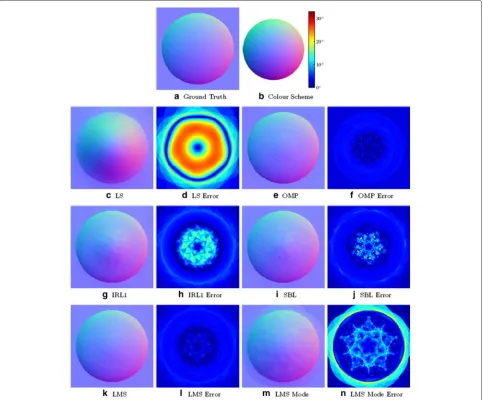
The effect of specularity on normal map recovery can be further seen from the results for the Spheredataset in Fig. 7. Again, IRL1 and SBL results are noisy in the specularity-affected areas, whereas OMP gives much cleaner results. LMS performs similarly to OMP. Interest-ingly, a pentagon-shaped pattern is visible on each error map because there are exactly five lights at each elevation angle.
Fig. 14Statistics for the angular error of normal maps recovered using sparse methods.Upper row: sample rendered images withphong_size
For Buddha (Fig. 8), OMP again produces a bet-ter overall result than IRL1 and SBL. However, the relatively poorer performance of the greedy methods in shadowed concave regions now becomes a more significant problem due to the prevalence of concave regions such as creases on the clothes. The angu-lar error distribution of the LMS result is simiangu-lar to that of OMP, though with slightly greater overall error.
From the normal map recovery results obtained on the three datasets, we can see that OMP generally performs better than IRL1 and SBL on convex objects and are more resistant to specularities and cast shadows. The statistical result of the angular error of the normal maps recovered with different methods are listed in Table 1. OMP result has the lowest mean, median, 25 % and 75 % quantiles, as well as standard deviation for all three datasets men-tioned above. The LMS result is better than IRL1 and SBL,
but worse than OMP. These results are also depicted in Fig. 9. Curiously, we notice that the estimation accuracy is generally lower onSpherethanCaesar, despite the simple geometry of the former. This may be jointly caused by the unique lighting model, surface colour and material that Sphere is rendered with. The exact explanation for this observation requires further investigation in the future.
As is witnessed on theBuddhadataset, OMP performs less optimally than IRL1 and SBL on small concave regions that are rarely illuminated. This problem also occurs for Caesar on the medial side of the eyes and under the
eyebrows. It is a lesser concern for objects that are gen-erally convex such asCaesarandBuddhabut may exert a strong negative influence on a scene that contains large concave areas. We will demonstrate the result for such a scene usingVenusin Section 4.2.2.
4.1.2 Comparison via reconstructed surfaces
Using the normal maps recovered with various methods, we also reconstructed the 3D surface with the Frankot-Chellapa method [73] for direct comparison of the shape. Here, only the reconstruction result for Caesar is used
for demonstration. It is apparent from Fig. 10 that in the LS, IRL1, and SBL results, the overall shape of the face appear to be more protruding then it actually is, espe-cially at the eyebrow ridge and the nose, whereas the OMP manages to preserve the shape accurately. Again, the LMS result appears to be less protruding than IRL1 and SBL results, although still not as accurate as OMP. We speculate that the exaggerated convexity originates from the inaccurately estimated normal vectors at high-light areas, such as the forehead and the nose. Since our greedy algorithm generally provides a better recovery in
those regions, they naturally yield a more accurate shape recovery.
4.1.3 Real datasets
Three datasets of real-world scenes are tested in this study:Gold, an ancient golden coin,Elba, an Italian high-relief sculpture, andFrag, a much-decorated golden frame (that surrounds a painting by Fragonard). Sample images of the three datasets are shown in Fig. 11.
The advantages and disadvantages of the methods we found using synthesized datasets are also observed in the
real datasets. Most images in dataset Goldhave a large area of cast shadow. The influence of shadow can be clearly seen on the normal maps recovered by LS, IRL1 and SBL (Fig. 12a (1–3)) but is completely eliminated by OMP (Fig. 12a (4)). As forElba, the scene contains a great number of small concave regions such as the pleats on the curtain. As expected, the greedy algorithm fail at these regions. Again, we notice that the LS, IRL1 and SBL results are more protruded than greedy results for bothGoldand Elba (Fig. 12a (1–5), b (1–5)). Although there is not a ground truth normal map to support our speculation, it is reasonable to argue that the non-greedy algorithms exag-gerate the convexity forElba, as was the case forCaesar
(Fig. 10). The complex geometry of the object in our third dataset—Frag—accounts for the noisy estimates observed in concave regions in the greedy normal maps (Fig. 12C4 and C5). Note that the non-greedy results also show a large degree of inaccuracy in these regions (Fig. 12C1– C3), but in a less noticeable manner since these artefacts are usually smoothly blended into less-affected areas.
4.1.4 MERL database
We also tested the performance of OMP on 95 materi-als from the MERL BRDF database [74]. Each material is rendered on a sphere at a resolution of 200×200 on 50 images of various lighting directions. The performance
pattern of OMP is very similar to SBL (Fig. 13): both methods are good at handling materials with an insignif-icant specular component (e.g. #10,red-specular-plastic). On the other hand, they both show decreased accu-racy on shiny, strongly non-Lambertian metallic materials (e.g. #90,silver-metallic-paint) probably due to the viola-tion of the sparsity assumpviola-tion. Overall, the mean angular error of OMP over all 95 materials is 6.3174°, on par with SBL (6.5370°), and both methods significantly outperform the naive LS (10.8027°).
4.2 Robustness
To further understand of how well these methods behave in the presence of non-Lambertian effects, we tested their performance onSpherewith varying degrees of specular-ity and on Venus, where a large portion of the scene is concave, and as such, is heavily polluted by cast shadow. To find out the robustness of these methods against exter-nal error introduced by the experimental setup, we also tested the methods with additive image noise and light calibration error.
4.2.1 Specularity
We rendered five datasets of the same object Sphere with various sizes of highlight area (Fig. 14, top row) and tested how the size of the specular region affects the performance of our sparse regression methods. The size of the highlight is controlled by the phong_size parameter in POV-Ray [72]. We found that although the accuracy of all three methods compared (IRL1, SBL, OMP) decreases as the specular size increases, the greedy algorithm is less affected (Fig. 14, middle and bottom figures).
4.2.2 Shadow and concavity: a failure case
In Section 4.1.1, we have already noticed the possibility that the performance of our greedy algorithm may be neg-atively affected at shadowed concave regions. Here, we use theVenusdataset to further demonstrate this observation. InVenus(Fig. 5, bottom row), the convex foreground (the Venus statue) and the concave background (the dome) are well separated, allowing us to clearly inspect the perfor-mance of algorithms on different regions.
The result is shown in Fig. 15. As speculated, OMP shows robustness in shiny, convex regions such as the outer rim of the dome, and on the statue itself, but fails on the heavily shadowed background. The other three methods (LS, IRL1, SBL), on the contrary, suffer from noticeable angular error in convex areas. However, they are less severely affected by shadow and concavity on the background than greedy methods. Overall, the normal map recovered with the greedy approach are less smooth for Venus due to the inaccurate estimation of normal vectors in the concave regions.
4.2.3 Image noise
We tested three sparse algorithms (IRL1, SBL and OMP) against Gaussian noise as well as salt and pepper noise. For Gaussian noise (Fig. 16), the accuracy of all three methods drastically decreases as the noise level increases, although OMP appears to be slightly more adversely affected. On the other hand, all sparse methods are quite insensitive to salt and pepper noise (Fig. 17).
4.2.4 Lighting
There might be cases when the lighting directions are not properly calibrated. That is, the assumed lighting direc-tions deviate from their actual values. In this test, we introduce for every assumed lighting vector a fixed angu-lar perturbation, ranging from 2° to 32°, at a random direction, while keeping the actual arrangement of lights unchanged.
We tested the performance of the sparse methods under various degrees of light calibration error on the Caesar dataset. The actual arrangement of lights is displayed in Fig. 18 (leftmost plot on the top row). As an increasingly greater random perturbation is added to the assumed lighting directions, the angular error gradually increases for all sparse methods. Note that OMP appears to be susceptible to the random calibration error the most, especially when the perturbation reaches 32°.
Also note that in Fig. 18 (bottom), the median of the angular error produced by OMP slightly decreases at 16◦ compared to previous conditions. We believe that this is a fluctuation caused by the particular arrangement of lights at this condition. Despite this decrease in the median of error, the widths of the error distributions steadily increase at 16◦for all three methods, as can be clearly seen from Fig. 18 (middle).
It was reported that the number of lights has a large impact on the accuracy of sparse photometric stereo recovery [2]. We found that our OMP-based method also shows a similar but somewhat greater dependency on the
number of lights (Fig. 19). This observation indicates that the OMP works best when a large number of lights are present.
We also investigated the performance of sparse meth-ods under a highly biased lighting distribution. We used 25 lights; 23 of them is located on the left or upper-left hemisphere and the other two on the right (Fig. 20). Under such a biased lighting, OMP still has the best mean angular error (8.2140°) compared with IRL1 (9.1173°), SBL (8.6561°) and LS (12.0726°).
4.3 Efficiency
The actual per-pixel processing time for the MATLAB implementation of the algorithms tested in this study is reported in Fig. 21. The maximum number of iterations for IRL1 and SBL are set to 100 although iteration will be terminated as soon as another stopping criterion is met; OMP always terminates after exactly 28 iterations for our datasets of 50 images; for LMS, the number of iterations is fixed at 1500.
In OMP, the operation with the highest asymptotic com-plexity is the inversion of a k × k matrix (where k is the number of selected columns) in Eq. 14. With a naive Gauss-Jordan elimination method, the inversion takes O(k3), which is asymptoticallyO(n3)sincek ≤ n/2+3. Since the above operation is repeatedn/2+3 times, the overall time complexity of our OMP algorithm isO(n4). In our current implementation, the running time of OMP (4.823 ms/pixel) is comparable to IRL1 (3.338 ms/pixel). LMS is the slowest (57.48 ms/pixel), though it can be made faster with fewer iterations at the expense of accuracy.
Fig. 20Recovery accuracy under highly biased lighting distribution. Polar plot shows the arrangement of lights. Upper and lower border ofblue boxesrepresent third (Q3) and first (Q1) quartiles, respectively.
Upper and lower whiskersshow 1.0 IQR extended from Q3 and Q1, respectively.Red bars in blue boxesrepresent medians
Fig. 21Average running time (per pixel) of photometric stereo algorithms measured in milliseconds
4.4 Summary
Based on the experimental results above, we have come to the conclusion that our greedy algorithm overall has a higher accuracy than L1 minimization and SBL with a comparable efficiency, though OMP may be less robust in poorly illuminated regions. LMS is close to the greedy sparse algorithm in accuracy, despite its low efficiency. The algorithms tested in this chapter are summarized and compared in Table 2.
5 Conclusions
In this study, the classical PST is reformulated in terms of the canonical form of sparse recovery, and a greedy algorithm—OMP—is applied to solve the problem. Our formulation is different from previous ones [1, 2] in that the former incorporates normal vector components and non-Lambertian errors in one combined vector, allowing for the straightforward application of OMP. In order for OMP to obtain normal estimations, the normal vector components have to be selected before the iteration stops. Although it is not theoretically guaranteed, we observed that the normal components are always selected within the first few iterations in the datasets we tested, unless some components are indeed zero or very close to zero. We also speculate that the dictionary matrix in our for-mulation is near-orthonormal and satisfies the conditions required by OMP to achieve exact recovery.
Table 2Qualitative comparison of photometric stereo algorithms
Robustness
Smoothness Efficiency
Overall Highlight Shadow Concavity
LS Very low Very low Very low Very low Very high Very high
LMS Very high Very high Very high – Low Very low
LMS mode Low Low Low – Medium Very high
IRL1 High High High Medium High High
SBL High High High Medium High Low
OMP Very high Very high Very high Low Medium High
The performance is evaluated on a five-level scale: ‘Very low’, ‘low’, ‘medium’, ‘high’ and ‘very high’. Fields that are not available are indicated by a ‘–’ sign
tested are reasonably robust against additive image noise and lighting calibration error.
Another two outlier-removal based methods—LMS and LMS mode finder—are also tested in this study for com-parison. LMS results are overall statistically more accurate than IRL1 and SBL but less so than OMP. LMS mode finder, the 1D simplification of LMS, shows some robust-ness against non-Lambertian errors, especially highlights but performs poorly against cast shadows.
This study opens up many possible directions for future research. First, a great number of sparse recov-ery algorithms have already been proposed in the past few decades, each designed for a specific formulation. Even within the domain of greedy algorithms, there are many other potential candidates aside from OMP that may be directly applied to the PST problem. It would be interesting to explore this large repertoire of sparse formulations and recovery algorithms to find an optimal method.
It has been shown that sparse methods such as IRL1 and SBL can be used to estimate the lighting directions in the context of uncalibrated PST [19]. It is highly pos-sible that greedy algorithms such as OMP can also be extended to be applied for such a purpose. Future stud-ies may reveal more applications of greedy algorithms in different aspects of the PST framework.
Competing interests
The authors declare that they have no competing interests.
Acknowledgements
The authors would like to thank the anonymous referees for their insightful comments and suggestions, which help improve the quality of the current study substantially.
Received: 7 April 2015 Accepted: 1 December 2015
References
1. L Wu, A Ganesh, B Shi, Y Matsushita, Y Wang, Y Ma, inProceedings of Asian Conference of Computer Vision. Robust photometric stereo via low-rank matrix completion and recovery (Springer, Berlin Heidelberg, 2010), pp. 703–717
2. S Ikehata, D Wipf, Y Matsushita, K Aizawa, inIEEE Conference on Computer Vision and Pattern Recognition. Robust photometric stereo using sparse
regression (IEEE Computer Society, Washington DC, USA, 2012), pp. 318–325
3. G Fyffe, X Yu, P Debevec, inInt. Conf. on Computational Photog. Single-shot photometric stereo by spectral multiplexing (IEEE Computer Society, Washington DC, USA, 2011), pp. 1–6
4. G Fyffe, P Debevec, inInt. Conf. on Computational Photog. Single-shot reflectance measurement from polarized color gradient illumination (IEEE Computer Society, Washington DC, USA, 2015)
5. A Hertzmann, SM Seitz, inIEEE Computer Society Conference on Computer Vision and Pattern Recognition. Shape and materials by example: a photometric stereo approach, vol. 1 (IEEE Computer Society, Washington DC, USA, 2003), pp. 533–540
6. N Alldrin, T Zickler, D Kriegman, inIEEE Conference on Computer Vision and Pattern Recognition. Photometric stereo with non-parametric and spatially-varying reflectance (IEEE, Anchorage AK, 2008), pp. 1–8 7. J Ackermann, M Ritz, A Stork, M Goesele, inTrends and Topics in Computer
Vision,Lecture Notes in Computer Science, ed. by KN Kutulakos. Removing the example from example-based photometric stereo (Springer, Berlin Heidelberg, 2012), pp. 197–210
8. F Verbiest, L Van Gool, in2008 IEEE Computer Society Conference on Computer Vision and Pattern Recognition. Photometric stereo with coherent outlier handling and confidence estimation (IEEE Computer Society, Washington DC, USA, 2008), pp. 1–8
9. C Hernandez, G Vogiatzis, R Cipolla, Multiview photometric stereo. IEEE Trans. Pattern Anal. Mach. Intell.30(3), 548–554 (2008)
10. MS Drew, Y Hel-Or, T Malzbender, N Hajari, Robust estimation of surface properties and interpolation of shadow/specularity components. Image Vis. Comput.30(4–5), 317–331 (2012)
11. M Zhang, MS Drew, inCPCV2012: European Conference on Computer Vision Workshop on Color and Photometry in Computer.Vision Lecture Notes in Computer Science. Robust luminance and chromaticity for matte regression in polynomial texture mapping, vol. 7584/2012 (Springer, Berlin Heidelberg, 2012), pp. 360–369
12. MS Drew, N Hajari, Y Hel-Or, T Malzbender, inProceedings of the British Machine Vision Conference. Specularity and shadow interpolation via robust polynomial texture maps, (2009), pp. 114–111411 13. DL Donoho, Compressed sensing. IEEE Trans. Inf. Theory.52(4),
1289–1306 (2006)
14. BK Natarajan, Sparse approximation solutions to linear systems. SIAM J. Comput.24(2), 227–234 (1995)
15. RJ Woodham, Photometric method for determining surface orientation from multiple images. Opt. Eng.19(1), 139–144 (1980)
16. S Barsky, M Petrou, The 4-source photometric stereo technique for three-dimensional surfaces in the presence of highlights and shadows. IEEE Trans. Pattern Anal. Mach Intell.25(10), 1239–1252 (2003) 17. H Rushmeier, G Taubin, A Guéziec, inProceedings of Eurographics
Workshop on Rendering. Applying shape from lighting variation to bump map capture, (1997), pp. 35–44
18. P Favaro, T Papadhimitri, A closed-form solution to uncalibrated photometric stereo via diffuse maxima. IEEE Conf. Computer Vision and Pattern Recognit.157(10), 821–828 (2012)