3D Imaging based on Depth Measurement Technologies

3D Imaging based on Depth Measurement

Technologies

Ni Chen1,† ID, Chao Zuo2,† ID, Edmund Y. Lam3 ID, and Byoungho Lee1,*

1 _{School of Electrical Engineering, Seoul National University, Gwanak-Gu Gwanakro 1, Seoul 151-744, Korea;} [email protected](N.C.); [email protected](B.L.)

2 _{Jiangsu Key Laboratory of Spectral Imaging & Intelligent Sense, Nanjing University of Science and} Technology, Nanjing, Jiangsu Province 210094, China; [email protected](C.Z.)

3 _{Department of Electrical and Electronic Engineering, The University of Hong Kong, Pokfulam, Hong Kong;} [email protected](E.L.)

* Correspondence: [email protected]; Tel.: +82-2-880-7245 † These authors contributed equally to this work.

Abstract: Three-dimensional (3D) imaging has attracted more and more interests because of its widespread applications, especially in information and life science. These techniques can be broadly divided into two types: ray-based and wavefront-based 3D imaging. Issues such as imaging quality and system complexity of these techniques limit the applications significantly, and therefore many investigations have focused on 3D imaging from depth measurements. This paper presents an overview of 3D imaging from depth measurements, and provides a summary of the connection between these the ray-based and wavefront-based 3D imaging techniques.

Keywords: Three-dimensional imaging; computational imaging; light field; holography; phase imaging

1. Introduction

0 50 100 150 200 250 300 350 400 450

N

um

be

r

of

pa

pe

rs

Year

Growth of 3D imaging research papers

Figure 1. Number of papers with a title containing “3D imaging” in Google Scholar [1] during the past decades.

Beyond the conventional two-dimensional (2D) imaging and photography, 3D imaging, which carries more information of the world, has a wide range of applications, particularly in the fields of life science [2] and information science [3]. Therefore, it has been attracting more and more attention in recent years [4,5]. Figure1shows the growth of 3D imaging related research papers during the past decades in Google Scholar [1], showing increasing interest in 3D imaging.

When we refer to 3D information, we usually mean that in addition to the 2D images, the depth or shape of the objects is also captured. The 3D information of an object is contained in the wave’s intensity

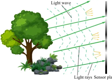
and phase of the light wave over it. 3D imaging, in some cases, can be regarded as both amplitude and phase imaging, which is also known as wavefront imaging. The phase of an electromagnetic wave is invisible, but it is inevitably changed as it passes through an object, which induces intensity changes. This can be illustrated in Fig.2. The shape of the object, including both the depth or surface, bents or distorts the light that goes through it. The amount of light bent behaves as phase delay, and reflects the surface topology [6] or the shape and density [7] of the object. The detected intensity image of the wavefront thus carries the 3D information of the object, resulting in specific intensity patterns. The brighter areas reflect light energy concentration and dimmer areas reflect light energy spreading out, as shown in Fig.2.

Light wave

Light rays Sensor plane Figure 2. Relationship between light ray and wave.

As is commonly known, light wave and ray are used to describe light in different levels, while Eikonal equation gives a link between ray optics and wave optics [8]. Wave optics is used to describe phenomena where diffraction and interference are important, while ray optics is where light can be considered to be a ray. In many imaging cases, treating light as ray is enough to solve the problems. From the viewpoint of ray optics, as shown in Fig.2, the directions of the reflected light rays are determined by the normal to the object surface at the incidence point [9]. Therefore, By recording the light rays coming from the objects with their directions, we can also reconstruct its 3D surface shape. Imaging with light rays along with its direction is called light field imaging [10,11]. In this paper, we name it as “light ray field” to distinguish from “light wavefront field”. Based on the above description, 3D imaging can be regarded as light ray and phase (wavefront) imaging to some extent.

The applications of 3D imaging are extremely wide. Figure 3shows several of them. The wavefront-based 3D imaging is efficient for viewing structures in microscopy [12] and medical applications. The light ray field, which can produce multiple view images with parallax, is a practical and commercialized way for both stereoscopic and auto-stereoscopic 3D displays [13,14]. Benefiting from 3D imaging, hologram synthesis, which sometimes combines the wavefront-based and ray-based light field techniques, can make a hologram of the real world 3D scene under incoherent illumination, making holographic 3D display more realizable [15,16].

Intensity Phase

(a)

Intensity Surface Profile

(b)

Hologram reconstruction Generated hologram Real 3D object

Depth Depth camera

(c)

Flat di splay pa

nel

3D image Lens array

(d)

Figure 3. Applications of 3D imaging for (a) microscopy, (b) surface measurement, (c) holographic display, and (d) light field display.

the two types respectively in Sections3and4. Due to the close connection of the ray and wave optics, there is no clear boundary between the two types of 3D imaging techniques. In Section5, we show comparisons between some of these techniques. Some concluding discussions are given in Section6.

2. Theory of 3D imaging and progress of its development

In this section, we describe the fundamentals of ray-based and wavefront-based 3D imaging respectively. It will reveal why 3D imaging with depth measurements becomes a trend.

2.1. Ray-based light field imaging

y

z

0

L(r, θ, z)

x

θ

(a)

Lens array Sensor

f_l

Δx

θ_max

Δs

(b)

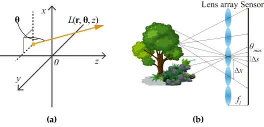
Figure 4. Light field (a) and its conventional capture (b).

As Fig.4(a) shows, according to the plenoptic function [28], light ray field can be parameterized as a functionL(r,θ,z)with its spatial position(r,z)and propagation directionθ, whereris the position vector representing the transverse spatial coordinates(x,y)andθis the propagation vector of(θx,θy).

that the energy traveling along the optical rays is a constant, the 2D images detected by a camera at a plane perpendicular to the optical axis atzccan be expressed by angularly integrating the the light rays

Ii(r,zc) = 1

z2

c

Z ∞

−∞L(r,θ,zc)dθ. (1)

The light ray field can also be easily propagated from a plane atzto another plane atz0by [30]

L(r,θ,z0) =L

r α+θ

1− 1

α

,θ,z

, (2)

wherez0 =αz, andαis a natural number. The transformation property of the light ray field makes it

useful for 3D imaging such as depth map reconstruction [31] and digital refocusing [30,30]. Besides, it is also an efficient way for glass-free 3D displays [13,14,32].

Various light ray field acquisition methods have been developed, including complicated setups such as camera arrays [33,34], compact designs that utilize micro-lens arrays [30,35], frequency domain multiplexing [35], amplitude masks [36,37], and well-designed mirrors [38,39]. Among these techniques, a camera with a micro-lens array in front of its sensor [30,40,41] is well-known and widely used due to its single-shot convenience, as Fig.4(b) shows. In this kind of capture, every micro-lens captures angular distribution of the light rays at its principal point. The number of light rays that can be recorded depends on the lens pitch∆xand the pixel pitch∆sof the camera sensor.

The maximum angleθmax of the light rays that can be collected depends on the focal length fland

the lens pitch∆x. The spatial sampling interval of the object is the same as the pitch of the lens array. This lens array based method enables direct capture of the light field at a single shot, but the spatial resolution and angular resolution of the captured light field mutually restrict each other [13,14]. This mutual restriction occurs in the similar setups like camera array. During the past 15 years, many techniques have been proposed to enhance the spatial resolution, the view angle and the expressible depth range [14,42–44]. Unfortunately, there is no way to eliminate these shortages that inherited from the array-like devices.

Based on the fact that depth measurements carry the 3D information of the objects, researchers have tended to retrieving light ray field from depth measurements instead of using arrays. We review these techniques in Section3.

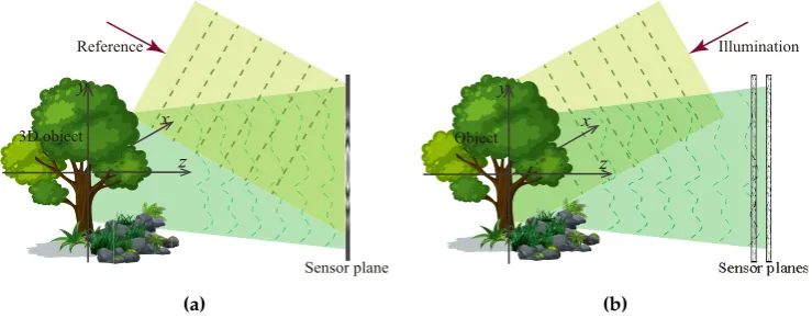
2.2. Wavefront-based light field imaging

x y

z 3D object

Reference

Sensor plane

(a)

x y

z Object

Illumination

(b)

Figure 5. Two typical wavefront imaging techniques: interferometric (a) and phase imaging (b).

imaging setup with depth measurements, as Fig.5(b) shows, which leads to a broader applications of phase imaging, such as X-ray imaging [50].

Phase retrieval usually can be achieved by iterative and quantitative approaches. Both only require one or a few depth measurements of the diffracted wave. In Section4, we will review this kind of techniques.

3. Ray-based light field imaging from depth measurements

In light ray field reconstruction, the depth measurements are usually detected by a conventional camera such as a digital single-lens reflex (DSLR), under white light source. The formation of the photographic images has a close connection to the light ray field under geometric optics, and we will show this in the following paragraphs. After this, we will review the related techniques.

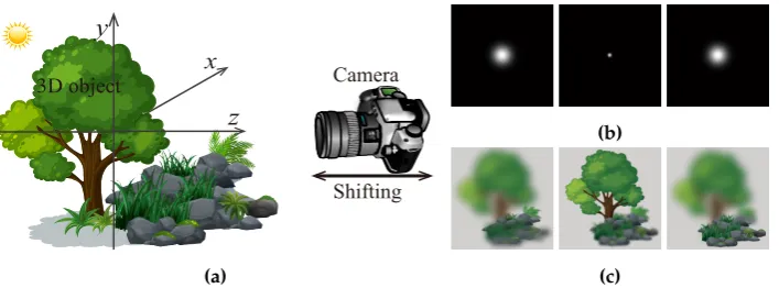
3.1. Focal sweeping measurement with a conventional camera

r

z

θ

L(r, θ₎

(r_+zθ_{, z)}

0

3D surface

r

Figure 6.A 3D object’s light field representation.

We start from considering a 3D object with its center located at the origin of the Cartesian coordinates. Suppose the center of the 3D objectO(r,z)is located at the origin of the coordinate system, and it is regarded as a stack of 2D slices, i.e.,O(r,z) = R

O(r,z). The light ray field representation of the 3D object with the principal plane located at its center can be expressed as the integral of the object’s projections by Fig.6with [51]

L(r,θ, 0) = Z

O(r+zθ,z)dz. (3)

Figure6shows the geometry relationship between the 3D object surface and its light ray field on the r–zsectional plane.

x

Shifting

y

z

Camera 3D object

(a)

(b)

(c)

Figure 7.Scheme of focal sweeping capture (a), and sample of the captured images of a point source (b) and a 3D scene (c).

of the object and the point spread function (PSF) of the system at the corresponding plane [52]. Mark Ii(r,zc)as a captured image at a plane ofzc, it thus can be expressed as

I_i(r,zc) =

Z

O(r,z)⊗hi(r,zc−z), (4)

where hi(r,z) is the PSF of an incoherent imaging system, and⊗ is the 2D convolution operator.

Since the aperture of a camera is usually circular, its PSF is approximately a 3D Gaussian distribution function which is symmetrical with respect to the focal plane along the optical axis [53,54]. Figure7(b) shows a sample of several simulated 2D slices of the 3D PSF in a conventional camera imaging system, and Fig.7(c) shows several sample images captured at different planes.

Because of Eq. (4), the early light ray field reconstruction algorithms from photographic images use image deconvolution, which is an inverse process of Eq. (4) [55]. However, the blur kernel, which is related to the PSF, requires dense sampling to build, and thus could not give good results when the number of samples is limited. Subsequently, techniques involving the insertion of coded masks into a camera have been invented to obtain a higher resolution light ray field [18,56]. Although they achieve a better resolution than the lens array based techniques, they sacrifice light transmission because of the masks. Besides, they usually require solving a computationally intensive inverse problem, often with prior knowledge of the object scene. All of these problems limit their applications [36,57].

In recent years, focal stack imaging has attracted a lot of attention [58]. Focal stack is well known as a tool for extended depth of field photography [59] and fluorescence tomography [60]. Researchers have reported that it is also possible to reconstruct a light ray field from a multi-focus image stack [61–63]. The reason why light ray field can be extracted from a focal stack is obvious, as the 3D information is stored in the stack. This can also be explained mathematically. It is due to the interchangeable property between light field and photographic images presented by Eqs. (4) and (1), which is fundamental to most light ray reconstruction techniques that are based on depth measurements. In such techniques, there is no need to mount or insert any additional optical elements to the camera, making it possible to capture a light ray field with commercial DSLR cameras.

In the following section, we give a review on this kind of techniques, especially the light field reconstruction with back projection (LFBP) approach [62,63] and the light field moment imaging (LFMI) [27,67].

3.2. Light ray field reconstruction by back-projection

Because of the interchangeable relationship between light ray field and 2D photographic images, the light field can be reconstructed from the depth measured photographic images directly by back-projection.

SupposeI_i(r,zq)is a photographic image taken atz=zq, andmis the index number of one image

in the photo stack. The total number of captured images is denoted asQ. With these captured images, the light field with the principal plane located atz = 0 is calculated by using the back-projection algorithm [62]

L(r,θ, 0) = 1 Q

Q

∑

q=1

I_i r+zqθ,zq. (5)

We call the light ray field reconstruction directly with this equation as LFBP I. Here, we neglect the magnification factor of the images. This is because the captured images can be aligned and resized easily with digital post-processing. Eq. (5) can be explained by Fig.8more intuitively. In Fig.8(a), a light rayL(r,θ, 0)with a propagation direction ofθcontributes to two different positions in the defocus images, in front of and behind it, i.e.,r1in the front image andr2in the real image. The positions can be obtained by the projection angle and the depth position of these images byrq=r+zqθ. Based on

this fact, the radiance of the light ray can be obtained by the average value of the pixels on all of the depth images along the ray directions.

z x

L(r_, θ_{, z} 0)

r z₂

z₁

y

r 2

r 1

(a) r1=θz1

z1

r z0

θ r

r2=θz2 z2

(b)

x

z

0

θ

x

θ

y

(c)

Figure 8. Principle of LFBP represented in the spatial domain (a) and by WDF (b), and an example of the reconstructed EPIs of a real 3D acene (c) (Adapted with permission from [66], [Optical Society of America]).

function (WDF) [68]. A ray with a fixed propagation angle corresponds to different shearing of the focused EPI, therefore, its radiance can be obtained by integrating over all the red points in the three EPI images, i.e., accumulation along the red dashed horizontal line. Figure8(c) shows an example of the LFBP I technique, where the left image shows the 3D object scene, and the upper right images are the captured images, whereas the bottom right images are the EPIs of the reconstructed light field. Since the captured images are not segmented by lens arrays, the reconstructed light ray field shows a better angular and spatial resolution, as reflected by the EPIs in Fig.8(c). The spatial image resolution is comparable to that of a conventional camera sensor. Note that the angular sampling of the light field calculated from the photographic images depends on the numerical aperture (NA) and the pixel pitch of the camera sensor, rather than the number of images captured along the optical axis.

As the EPIs shown in Fig.8(c), the light field reconstructed with this approach has a severe noise problem [62,66,69]. The EPIs show overlap, and this phenomenon is very serious when the 3D scene is complicated. Chenet al.have analyzed this noise by giving the exact expression of the LFBP that relates to the depth measurements [51]

L0(r,θ) =

Q

∑

q=1

O(r+zqθ,zq) + Q

∑

q=1 Z

z6=zq

O(r+zqθ,z)⊗hi(r+zqθ,zq−z)dz. (6)

Since a 3D objectO(r,z)can be discretized along the optical axis byO(r,z)≈∑N

n=1O(r,zn), whereNis the slice number, Eq. (3) can be rewritten asL(r,θ) =_∑nN₌₁O(r+znθ,zn). Therefore, whenQin Eq. (6)

approachesN, the first term approaches Eq. (3), which corresponds to the discrete approximation of the 3D objects’ light field. WhenQis much smaller than N, it is equivalent to axially sampling the object insufficiently, which affects the depth resolution of the reconstructed light field. The second term of Eq. (6) is noise. Obviously, it is the accumulation of the defocus noise induced by the images of the object slices which are out of focus. From this equation, we can see that there are two main parameters affecting the noise: the number of depth images and the PSF of the camera. The PSF is related to the f-number of the camera, i.e., the NA. As the second term of Eq. (6) shows, for the LFBP technique, smaller NA and fewer images produce higher quality reconstructed light ray field. However, to maintain the depth resolution of the reconstructed light field, the number of the captured images should be large enough. This mutual constraint property makes it difficult to get a high-quality light field with the conventional LFBP technique. This can be observed from the original paper [62] and the EPIs of Figs.9(a) and (c).

N=3 N=5 N=9 N=17

(a)

(b)

NA=0.2 NA=0.4 NA=0.6 NA=0.8

(c)

(d)

Figure 9.The reconstructed EPIs calculated from various number of depth images (a)(b) and 5 depth images captured under various camera NAs (c)(d), by the conventional LFBP I (a)(c) and denoised LFBP II (b)(d) respectively. (Adapted with permission from [51], [Optical Society of America].)

restructuring the 3D model firstly, then represent it with Eq. (3). Hence, it is very dependent on the depth map calculation algorithm. For comparison, we name the above two improved LFBP techniques as LFBP II [51,63].

3.3. Iterative light ray field reconstruction based on back-projection

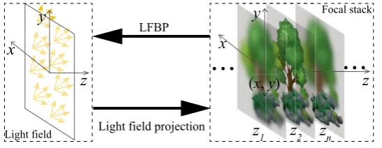
In order to obtain a more realistic light ray field reconstruction with higher quality, iterative light ray field reconstruction based on back-projection (iLFBP) techniques has been reported [71,72]. This kind of techniques are based on the fact of the interchangeable property between 2D camera images and the light ray field, which is indicated by Eqs. (1) and (5). Based on this imaging geometry, both Yin et al. and Liuet al. have reported an iterative light ray field reconstruction technique from focal stack measurements [71,72]. Their methods share the same concept.

Light field

z

z

z

z

x

(

x

,

y

)

y

x

y

z

z

Figure 10. Scheme of iLFBP.

In iLFBP, there is a projection bounce between the 2D focus stack images and the light ray field. For each bounce, a constraint related to the NA of the camera is applied. This is akin to the famous iterative phase retrieval algorithms that we will introduce in Section4.1. Instead of using the LFBP I, a more sophisticated filtered back-projection algorithm [72] or a Landweber iterative scheme [71] is used to project measured focal stack images to light ray field. This can make the best use of the structural information of the focal stack.

Since this kind of technique does not rely on a preprocessing or the complex nonlinear depth estimation process like in LFBP II, it is not affected by the accuracy of the depth estimation. The experiments show the advantages of this kind of techniques in accuracy, reduced sampling, and occluded boundaries. However, as all the other iterative based techniques, this kind of techniques is heavily time consuming.

3.4. Light field moment imaging

As we illustrated in the previous context, 3D information is carried by the photographic stack images. Even though the light ray field can be reconstructed by LFBP I and LFBP II, the depth resolution is closely related to the axial sampling induced by the depth measurements. Although the iLFBP shows possibility to use fewer images, it still requires quite a lot.

Motivated by the fact of light energy flow along the optical axis is reflected by the sweeping captured images, Orth and Crozier [27] have found that the angular moment of light rays satisfies a Poisson equation:

∂Ii(r,z)

∂z =−∇⊥· ∇U(r,z) (7)

implemented by using conventional cameras. The angular moment is then used to reconstruct 3D perspective views of a scene by [27]

L(r,θ,z) =I_i(r,z)exp

−[θ−M(r)] 2

σ2

=Ii(r,z)δ[θ−M(r)]⊗G(θ,σ), (8)

whereG(θ,σ)is the Gaussian function with standard deviationσ, which equals to the NA of the

system. This is based on the fact that the angular of the light rays satisfy Gaussian function [27], and can be modified properly when the camera used in the capture has a different aperture shape.

I

(

r

,

z

)

y

x

I

(

r

,

z

)

M(r1)

(r2)

M

(a)

Intensity r

1

r r₂

A

n

gl

e

r 1

r r₂

=

θ

θ

M(r1)

M(r2)

M(r1)

M(r2)

A

n

gl

e

(b)

(c)

Figure 11. Principle of LFMI represented in the spatial domain (a) and WDF (b), and one example of different view images reconstructed by it (c) (Adapted with permission from [64], [Optical Society of America].).

The theory of LFMI can be explained more intuitively by Fig.11. Fig.11(b) represents the LFMI calculation process in one dimensional (1D) EPI expression. The estimated angular moment represents the average light ray propagation direction at each spatial position, as shown in Fig.11(a), thus can be represented as a curve in 1D EPI, as the left image in Fig.11(b) shows, which corresponds to I_i(rn)δ[θ−M(rn)]in Eq. (8). The final calculated EPI (Right image in Fig.11(b)) is the convolution

between the angular moment and the Gaussian PSF (Center image in Fig.11(b)). It can be seen that the final EPI is mainly determined by the angular moment, whose accuracy affects the reconstructed light field the most.

LFMI has a counterpart in the wave-optics regime, the transport of intensity equation (TIE), which is a very effective tool for non-interferometric phase retrieval [74]. The key of LFMI is to obtain the first angular moment by solving a Poisson equation that is similar with TIE [27]. Thus, performance is very critical to the axial spacing between adjacent measurement planes [75,76]. Therefore, this axial spacing should be chosen carefully according to the object’s characteristics in order to obtain a good estimation of intensity derivative [27]. The estimation accuracy can be further improved with multiple images [67,73]. This issue is precisely identical to the noise-resolution tradeoff in TIE, which will be discussed in detail in Section4.2.3

perspective view like images. But it provides a new view on depth measurement based light ray field reconstruction, and is still useful for viewing 3D shape of small objects in some extent. More detailed discussions about the relationship between FLMI and TIE can be found in Section5.2.

3.5. Issues

Table 1.Comparison of light ray field reconstruction techniques.

Accuracy Noise Occlusion Time cost LFBP Ia Moderate High Exist Low LFBP IIb Moderate Low Exist partiale High iLFBPc High Low Exist less High

LFMId Low High Exist Low

a_[62],b_[51,63],c_[71,77],d_[27].

e_{Occlusion exist in [51] and does not exist in [63].}

In this section, we have introduced techniques of light ray field calculation from a series of depth images. Not being segmented by an array device, the spatial resolution is only limited by the camera NA as in conventional photography. As these methods do not require any special equipments like lens array or code masks, they are easy to be implemented. However, they have their issues. Table1 shows the comparison of these techniques. LFBP based methods can reconstruct the light ray field with defocus noise [62], which can be reduced by preprocessing [51,63] or iterative approaches [71, 72]. However, iteration makes the digital reconstruction time consuming. LFMI [27] reconstruct view like images by estimating the first angular moment of the light rays instead of exact light ray field with at least only two depth measurements, more exact reconstruction may need more depth measurements [67].

Lens

Pupil

Lens

Object

Objective

SLM

Lens Pupil Lens

Mirror Pupil Lens CCD

(a) (b)

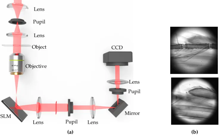
Figure 12. System setup (a) and two of the captured out of focus images (b) of the fast light ray field acquisition with PSF modulation (Adapted with permission from [64], [Optical Society of America].).

acquisition technique by using a spatial light modulator (SLM) to obtain defocussing instead of mechanical translation [64]. This technique can achieve fast data acquisition and is free of mechanical instability. The modulation is implemented in a microscopy imaging system, as Fig.12shows. With this system, the time cost for capturing a large amount of focal plane sweeping images is efficiently reduced. And the accuracy of the captured images is increased because there is no mechanical movement during the capture process. This technique may also be used to achieve other types of PSF distribution functions rather than Gaussian. In this case, the Gaussian distribution function in the LFMI equation should be modified to the corresponding PSF function. The microscopic imaging system can also be extended to conventional digital imaging system by using an electrically tunable lens [78] for colorful imaging.

4. Wavefront-based light field imaging from depth measurements

Phase retrieval based wavefront reconstruction techniques does not require any reference beam. Generally, one or several diffracted intensity images and some post digital image processing are needed. This kind of techniques are usually implemented by either iterative or deterministic approaches. Iterative phase retrieval techniques are based on the Gerchberg-Saxton (GS) method [79], and the deterministic approach usually means the TIE [74,80,81]. In the following we review these two types of phase retrieval sequentially.

4.1. Iterative phase retrieval

Image constraints Object constraints

P

P-1

Object plane Image plane

(a)

Image constraints Object constraints

… Δz

c,1 P₁

P1 -1

P2 Pm

-1

Pm

P2 -1

P_1,2

P_1,2 P1,m

P_1,m-1 -1

Δz c,m

Object plane

Image plane

(b)

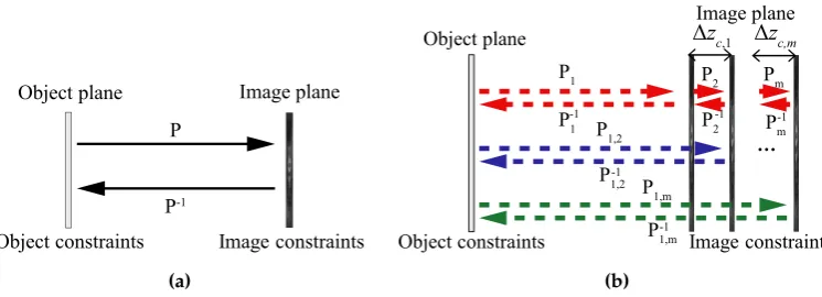
Figure 13. Iterative phase retrieval with (a) one single and (b) multiple depth measurements.

Almost all of the iterative phase retrieval techniques are based on the GS [79] and Yang-Gu (YG) [82] algorithms, which use prior knowledges of the object as constraints [19]. In the GS method, bounces between in-focus and Fourier domain images are performed, as shown in Fig.13(a),P andP−1is a pair of wave propagation operators. At each step, an estimation of the complex-field is updated with measured or a priori information of the object [19,83,84]. In this case, the accuracy of the phase retrieval is an issue. Phase solutions with this techniques are not unique, but are likely to be correct [85]. Besides, the stagnation of the iteration, and the local minimal problem have limited its application. Many techniques have been proposed for lessening the solution error [86] since this technique was invented.

Fresnel transformed images can also be used instead of Fourier transformed images [87], i.e.,P andP−1can be either Fourier transform or Fresnel Transform. The Fresnel transformation between the object and measurement planes instead of Fourier transform was a milestone. This makes the iterations not only be confined between object and image plane, but among multiple diffracted intensity images. The iteration among the object and the measurements can have many combinations, as Fig.13(b) shows. Bounces can be performed for all of the planes in one loop through the path ofP1 → P2· · ·Pm → Pm−1· · · → P2−1 → P

−1

performed only among the measurements. As a result, the prior knowledge about the object became unnecessary. Multiple measurements have improved the accuracy of the phase retrieval and the unnecessary object prior requirement, result in a broader application of iterative phase retrieval [88,89].

In the past decades, research about the iterative algorithm, defocus of the measurements, light modulation, multiple measurements have been fully studied. Fienup has reported the gradient decent search (GDS) algorithm and hybrid input-output (HIO) algorithm successively [19], where the IO has been proved to be very effective and is widely used up to now.

Except improvement on the algorithm, the required properties of the measurements, which represent the image constraints have also been studied. It has been demonstrated that the accuracy of the phase reconstruction is affected by the defocus amount of the measured images [87,90], which is object-dependent. Large propagation distance usually produces better diffraction contrast, thus makes these techniques work better for X-ray imaging [91,92]. A known illumination pattern used as a constraint can eliminate the prior knowledge requirement [89]. A random amplitude mask [93] or random phase plate [94,95] used to modulate the illumination, requires less iterations for reconstruction because the low frequencies of the object are transformed to fast varying high frequencies. The induced problems by these techniques are, an amplitude mask resulting in the diminution of light energy and the use of a phase plate requires difficult fabrication.

Multiple measurements can also be regarded as improving of the object constraint to some extent. Because multiple measurements with variations in depth detect spatial frequencies at different sensitivities [88,96–99], thus they can also improve the resolution of the reconstruction. Multiple depth measurements can be produced by capturing intensity images under illumination with different wavelengths at a single position [100], or under a single beam illumination with different foci [88], translating an aperture transversely [96]. Except for depth measurements, other types of multiple measurements, such as off-axis multiple measurements of synthetic aperture (SA) [101,102], ptychographic [101–104], and structured illumination [105,106] have been proven more efficient in image quality.

The significant amount of the data carried by multiple measurements makes the phase retrieval very robust and rather stable to noise [50]. It is obvious that more measurements result in higher quality reconstructions [107]. However, capturing more intensity images requires more movement steps of the camera or the object, which makes the captured images sensitive to small misalignments in the experimental setup, thus the noise induced to the captured intensity images becomes more serious. Besides, time consuming of the capture makes it not capable for use in dynamic object or real-time applications. To improve the multiple measurement capture [98], beam splitters [50], SLM [108,109], and deformable mirror (DM) [110] were used to achieve single-shot/single-plane measurements. However, beam splitter causes light attenuation, and the use of SLM or DM sacrifices the simplicity of the experimental setup. All of these approaches require additional optical components and involve complicated post digital processes. Therefore, algorithms based on multiple measurements have also been developed on the other hand [99].

The typical iterative phase retrieval techniques are summarized in Table 2. Despite of the limitations of each technique, the iterative phase retrieval remains as a popular technique for wavefront reconstructions due to the fact that the optimal transfer function is object-dependent and the simplicity of its implementation. However, iterative phase retrieval based on scalar diffraction theory [52] works under coherent illumination, which limits its application. TIE, which is presented in the next section of 4.2, has been proved as a compensation to iterative phase retrieval technique.

4.2. Transport of intensity equation

Table 2.Comparison of iterative phase retrieval techniques

Techniques Pros Cons

Algorithm

GS 2 images

Error Stagnation Local minima

GDS Moderate fast low

IO Effective

Contraints

Amplitude mask Fewer iteration Attenuation

Phase mask Fewer iteration Fabrication

Known pattern Fewer iteration

Multi-depth Resolution Time cost

Single position/shot possible Possible experimental complexity

Multi-wavelength Resolution Time cost

Single position Expensive

Multi-angular Resolution Experimental complexity Structure illumination Resolution Experimental complexity Synthetic Aperture Resolution Experimental complexity

advancements in optical microscopy and digital signal processing have brought TIE back to the forefront of quantitative phase microscopy [115–118] and 3D depth imaging [27,64,119]. The TIE specifies the relationship between object-plane phase and the first derivative of intensity with respect to the optical axis in the near Fresnel region, yielding a compact equation which allows direct recovery of phase information [21]

−k∂I(r)

∂z =∇ ·[I(r)∇

φ(r)], (9)

where k is the wave number 2π/λ, r is the position vector representing the transverse spatial

coordinates (x,y). ∇ is the gradient operator over r, which is normal to the beam propagation directionz.I(r)is the intensity, located without loss of generality at the planez=0, andφ(r)is the

phase to be retrieved. Expanding the right hand side (RHS) of Eq. (9), one obtains

−k∂I(r)

∂z =∇I(r)· ∇

φ(r) +I(r)∇2φ(r). (10)

In the above expression, the first term on RHS is called prism term, which stands for the longitude intensity variation due to the local wavefront slope. The second term on RHS is called lens term representing the intensity variation caused by the local wavefront curvature. It can be seen that TIE links the longitudinal intensity derivative with the slope and curvature of the wavefront which produces the change in intensity as the wavefront propagates.

4.2.1. Solutions to TIE

TIE is a second order elliptic partial differential equation for the phase function, and solving this equation does not appear to be difficult. SupposingI(r)>0within enclosure ¯Ωand with appropriate boundary conditions (defined on the region boundary∂Ω), the solution to the TIE is known to exist

and be unique (or unique apart from an arbitrary additive constant) [80], i.e., the phase φ(r)can

be uniquely determined by solving the TIE with the measured intensityI and the axial intensity derivative∂I/∂z. The TIE is conventionally solved under the so-called “Teague’s assumption” so

that the transverse fluxI ∇φis conservative and can be fully characterized by a scalar potentialψ(an

auxiliary function):

Then the TIE can be converted into the following two Poisson’s equations:

−k∂I

∂z =∇

2

ψ, (12)

and

∇ ·(I−1∇ψ) =∇2φ. (13)

Solving these two Poisson’s equations is straightforward mathematically, and several numerical solvers have been proposed, such as the Green’s function method [21,120], the multi-grid method [121,122], the Zernike polynomial expansion method [123,124], the fast Fourier transform (FFT) method [81,121, 124,125], the discrete cosine transform (DCT) method [126,127], and the iterative DCT method [128].

Table 3.Comparison of TIE techniques

Issues Techniques Pros Cons

TIE solvers

Green’s functiona _{Theoretical analysis} Computation-extensive, memory-demanding

Multi-Gridb _{Simple and fast Low-frequency noise,}

Zernike polynomialsc

Precisely represent the optical aberration

only for circular regions, difficult to follow details

FFTd Fast, easy to implement, incorporate regularization in reconstruction

Imply periodic boundary conditions

DCTe Fast, inhomogeneous

Neumann boundary condition

Rectangular aperture, required to limit FOV

Iterative DCTf Inhomogeneous Neumann boundary

condition, arbitrarily shaped apertures Need several iterations

Boundary conditions

Homogeneous Dirichlet/Neumanng

Easy to apply, can be

implemented by different solvers “Flat” boundary phase

Periodich Can be implemented by

FFT-based solver Periodic boundary phase Inhomogeneous

Dirichleti - Boundary phase required

Inhomogeneous Neumannj

Can be measured by

introducing a hard aperture -Phase

discrepancy

Picard-type iterationk

Can compensate the phase

discrepancy Need 2-4 iterations

Axial derivation

2-planesl Less intensity acquisition Noise-resolution trade off

Multi-planesm Higher resolution,

better noise tolerance More measurements a_[21,120],b_[121,122],c_[123,124],d_{[81,121,124,125],}e_[126,127],f_[128],g_[129,130],h_{[81,121,124,125],}i_[21],

j _[126–128],k_[131],l_[21],m_[132–142]

Despite its mathematical well-possessedness, the rigorous implementation of the TIE phase retrieval tends to be difficult because the associated boundary conditions are difficult to measure or to know as a priori. Figure14shows three typical boundary conditions used in TIE solvers: Dirichlet boundary conditions, Neumann boundary conditions, and periodic boundary conditions. Since the phase function is exactly the quantity to be recovered, its valueφ|_∂Ω (for Dirichlet boundary

condition) or normal derivativeI∂φ/∂n|_∂Ω(for Neumann boundary condition) at the region where

(a) (b) (c)

Figure 14. Three typical boundary conditions used in TIE solvers: (a) Dirichlet boundary conditions (need to know the phase value at the boundary), (b) Neumann boundary conditions (need to know the phase normal derivative at the boundary), and (c) periodic boundary conditions (assume the object is periodically extended at the boundary).

129,130,143]. Coincidentally, all the efforts aim to find some ways to nullify the overall energy transfer across the region boundary, making boundary conditions unnecessary

Z Z

Ω

∂I(r)

∂n dr=0. (14)

(a)

(b)

(c)

Figure 15.Phase retrieval simulations for different types of objects: (a) An isolated object located in the central FOV (FFT-based solver gives accurate reconstruction), (b) a complex object extending outside the image boundary (FFT-based solver produces large boundary artifacts), and (c) DCT solver with a hard aperture (the inhomogeneous boundary conditions can be measured at the boundary, which produces accurate phase reconstruction even if the object is located at the aperture boundary).

One simple and common way to satisfy this condition is to let the measured sample be isolatedly placed in the center of the camera field of view (FOV), surrounded by an unperturbed plane wave (the phase is “flat” at the boundary of the FOV), in which case the energy (intensity) conservation is fulfilled inside the FOV at different image recording locations, as shown in Fig.15(a). Then one can safely define some simplified boundary conditions,e.g., the homogeneous Dirichlet conditions (zero phase changes at the boundaryφ|_∂Ω =C, whereCis a constant), the homogeneous Neumann boundary conditions

(constant phase at the boundaryI∂φ/∂n|_∂Ω =0), or the periodic boundary conditions (the phase at the

experimental conditions. When the actual experimental condition violates those imposed assumptions, e.g., in wavefront sensing (non-fact phase at the boundary) or objects extending outside the image boundary, as shown in Fig.15(b), severe boundary artifacts will appear, and seriously affect the accuracy of the phase reconstruction [129,130,143].

To bypass the difficulty in obtaining real boundary conditions, Gureyev and Nugent [124] suggested another way to eliminate the need of boundary conditions by considering the special case that the intensityI > 0 inside the domainΩbut strictly vanishes at the boundary (so that I∂φ/∂n|_∂Ω = 0). Alternatively, without any additional requirement about the test object and

experimental conditions, Volkovet al.[129] proposed a pure mathematical trick to nullify the energy flow across the boundary through appropriate symmetrization of input images. However, it assumes there is no energy dissipation through the image boundary for any objects, which is generally not physically grounded. To summarize,’without boundary value measurements’ does not mean that the TIE can be solved without imposing any boundary conditions, or more exactly, we have to confine our measured object or experimental configuration to certain implicit boundary conditions.

For more general cases, as shown in Fig.15(b), the energy inside the FOV is not conserved, as energy “leak” occurs at the FOV boundary while the recording distance is being changed. In this case, inhomogeneous boundary conditions are thus necessary for the correct phase reconstruction based on TIE. Zuoet al.[126] addressed the solution of the TIE in the case ofinhomogeneous Neumann boundary conditionsunder nonuniform illuminations. By introducing a hard aperture to limit the wavefield under test, as shown in Fig.15(c), the energy conservation can be satisfied, and the inhomogeneous Neumann boundary valuesI∂φ/∂n|_∂Ωare directly accessible around the aperture edge. In the case

ofrectangular aperture, the DCT can be used to solve the TIE effectively and efficiently, which has been well demonstrated in application of microlens characterization [127]. Huanget al.[128] further extended the DCT solver to anarbitrarily shaped apertureby iterative compensation mechanism. Recently, Ishizukaet al.[144,145] successfully applied the iterative DCT solver to recover the additional phase term corresponding to the curvature of field on the image plane in TEM.

Helmholtz decomposition

Teague’s assumption Missing term

Transverse flux vector Gradient field Rotational field

x

y

4.2.2. Phase discrepancy and compensation

Another notable issue regarding the solution of the TIE is “phase discrepancy” resulting from the introduction of the Teague’s auxiliary function [21], which suggests that the transverse flux is conservative so that a scalar potentialψexists that satisfy Eq. (11). However, it is important to remark

that the Teague’s auxiliary function does not always exist in practical situations since the transverse energy flux may not be conservative, and consequently it would produce results that would not adequately match the exact solution [146]. This problem was first pointed out by Allenet al.[121] in 2001. Ten years later, Schmalzet al.[146] made a detailed theoretical analysis on this problem based on Helmholtz decomposition theorem and decompose the transverse flux in terms of the gradient of a scalar potentialψand the curl of a vector potentialη:

I ∇φ=∇ψ+∇ ×η. (15)

Compared with Eq. (12), it is plain to see that the term∇ ×ηis ignored in Teague’s assumption,

making a silent hypothesis that the transverse flux is irrotational (see Fig.16). In 2014, Zuoet al.[131] examined the effect of the missing rotational term on phase reconstruction, and derived the necessary and sufficient condition for the validity of Teague’s assumption:

∇I−1× ∇−2[∇ ·(∇I × ∇φ)] =0. (16)

Equation (16) shows that if the in-focus intensity distribution is nearly uniform, the phase discrepancy resulting from the Teague’s auxiliary function is quite small(∇I−1× ∇−2[∇ ·(∇I × ∇φ)] ≈ 0).

However, when the measured sample exhibits strong absorption, the phase discrepancy may be relatively large and cannot be neglected [146,147]. To compensate the phase discrepancy owing to Teague’s assumption, Zuoet al.[131] further developed a simple Picard-type iterative algorithm [131], in which the phase is gradually accumulated until a self-consistent solution is obtained. Within two to four iterations, the phase discrepancy can be reduced to a negligible level, and the exact solution to the TIE can be thus obtained.

4.2.3. Axial intensity derivative estimation

From the previous section, we know that in order to solve the TIE, one need to know the intensity I and axial intensity derivative∂I/∂z. Experimentally, the in-focus intensityI is easy to obtain.

However, the intensity derivative along the optical axis cannot be directly measured. Conventionally, it is estimated by a finite difference between two out-of-focus images, recorded symmetrically about the in-focus plane with±∆zdefocus distances [21], as illustrated in Fig.17(a).

∂I(r)

∂z ≈

I_∆z(r)− I−∆z(r)

2∆z . (17)

Mathematically, this approximation is valid in the limit of small defocus distances, where the error is the second order of the focus distance if the data are noise-free. However, experimentally the derivative estimate will become quite unstable when the distance∆zis too small because of the noise and quantization error [137]. On the other hand, increasing the two-plane separation∆zprovides better signal-to-noise ratio (SNR) in the derivative estimate, but the breakdown of the linear approximation induces nonlinearity errors, which results in loss of high frequency details [135]. Thus a compromise has to be made where∆zis chosen to balance the non-linearity error and the noise effect [148]. Specifically, the optimal∆zis dependent on both the maximum physically significant frequency of the object and the noise level [148,149]. However,a prioriknowledge about these two aspects is difficult to be known in advance.

Sample Imaging system Images

-∆z 0 ∆z -2∆z-∆z 0 ∆z2∆z

(a)

Sample Imaging system Multiple images

(b)

Figure 17. Typical experimential setup for TIE phase retrieval. (a) Conventional 3-plane TIE; (b) Multi-plane TIE. The through-focus intensity stack can be acquired by moving either the object or the image sensor.

in Fig.17(b), with more intensity measurementsIj∆z(r),j = −n, ...,−1, 0, 1, ...,n, the longitudinal

intensity derivative can be represented by their linear combination:

∂I(r)

∂z ≈

n

∑

j=−n

ajIj∆z(r)

∆z . (18)

Thus, it offers more flexibility for improving the accuracy and noise resistance in derivative estimation. Numerous finite difference methods have been proposed: such as high-order finite difference method [132,134,135,150], noise-reduction finite difference [133,151], higher order finite difference with noise-reduction method [136], and least-squares fitting method [135]. The only difference in these multiple planes derivative estimation methods lies in the coefficientsajin Eq. (18), and it has been found

that all these methods can be unified into Savitzky-Golay differentiation filter (SGDF) [152–154] with different degrees if the finite difference (Eq. (18)) is viewed from the viewpoint of digital filter [137]. Different from these finite difference methods with a fixed degree, methods that decompose the phase in the spatial frequency domain and estimate each Fourier component of the zderivative with an appropriately chosen finite difference approximation are particularly effective because they can balance the effects of noise and diffraction induced nonlinearity over a wide range of spatial frequencies [137–140]. For example, the optimal frequency selection (OFS) scheme proposed by Zuoet al.[137], uses a complementary filter bank in spatial frequency domain to select the optimal frequency components of the reconstructed phases based on SGDFs with different degrees to produce a composite phase image. Martinez-Carranzaet al.[139] extended the idea of multi-filter and frequency selection to accommodate the conventional three-plane TIE solver. Jenkinset al. [141] extended the basic principles of the multi-filter phase imaging to the important practical case of partially spatially coherent illumination from an extended incoherent source. Falaggiset al.[75] found that the optimum measurement distances obtained by multi-plane phase retrieval form a geometric series that maximizes the range of spatial frequencies to be recovered using a minimum number of planes. This strategy has been successfully implemented in the Gaussian Process regression TIE (GP-TIE) [142] and optimum frequency combination TIE (OFC-TIE) approaches [140], providing high accuracy of phase reconstruction with a significantly reduced number of intensity measurements.

to quantitative phase imaging: diminished speckle effects due to partially coherent illumination, and multimodal investigation potential due to overlaying with other modalities of the microscope (e.g. fluorescence, DIC, phase contrast). More recently, it has been found that the shape of the illumination aperture has a significant impact on the lateral resolution and noise sensitivity of TIE reconstruction [160–163], and by simply replacing the conventional circular illumination aperture with an annular one, high-resolution low-noise phase imaging can be achieved by using only 3-plane intensity measurements [160,161].

Collector Lens Aperture diaphragm Condenser

Sample

Objective

Conventional microscope

Tube lens _OL/ETL

TL -TIE add -on Module

Lens Lens

Camera

Electrically tunable lens

Collector Lens Aperture diaphragm Condenser

Sample

Objective

Conventional microscope

Tube lens

(a) (b)

SLM

SLM Mirror

Lens

Aperture

Lens Image

Plane ImagePlane

Lens

2fsinθ

Mirror

Figure 18.Advanced experimential setups for dynamic TIE phase imaging, which can be implemented as a simple add-on module to a conventional microscope. (a) Electrically tunable lens based TIE microscopy system (TL-TIE, figure adapted with permission from [78] ); (b) single-shot TIE system based on a SLM (SQPM, figure adapted with permission from [118]).

4.3. Discussions

Iterative phase retrieval and TIE are both important propagation-based phase imaging techniques, in which the phase contrast is formed by letting the wavefield propagate in free space after interaction with the object. TIE is valid under paraxial approximation and in the limit of small propagation distances (near-Fresnel region). The iterative phase retrieval is less restrictive, which does not rely on paraxial approximation, and is valid for both small and large propagation distances. However, it can sometimes exhibit slow convergence, and stagnation problems described in Section4.1. TIE is based on solving the intensity transport along the optical wave propagation, which does not explicitly resort to the scalar diffraction theory and does not need iterative reconstruction (deterministic). Besides, it generally requires less intensity measurements than iterative phase retrieval, and can directly recover the absolute phase without requiring phase unwrapping [116,164,165]. Thus, the complexity associated with the 2D phase unwrapping can be bypassed. More importantly, as will be introduced in Section5.2, TIE is still valid for partially coherent illumination [81,166–169], making it suitable for use in a bright-field microscope [115–118]. However, TIE has its inherent limitations as a tool for quantitatuve phase retrieval, such as the requirement of small defocus, paraxial approximation, and the inaccurate solutions induced by Teague’s assumption and inappropriate boundary conditions.

convergence of iterative methods can be significantly improved and the stagnation problems associated with the Gerchberg-Saxton-type iterative algorithm can be effectively avoided.

5. Ray-based vs. wave-based light field imaging

Due to the close connection of the ray and wave optics [8], 3D imaging techniques based on these two theories share many commons. Yamaguchi regards phase of a wavefront as a contribution to the resolution of light ray field [4]. This can be comprehended intuitively from Fig.2to some extent. Direction of light rays are along the normal of the wavefront, which is kind of sparse sampling of the continues wavefront in physical world.

The close connection between wavefront and light rays reflected by many techniques, such as Shack-Hartmann wavefront sensor and light ray field imaging with lens array, the TIE and LFMI. There are also many techniques that take advantage of this fact, such as synthesized hologram from multiple view images [175], hybrid approaches like holographic stereogram [176,177], and 3D Fourier ptychographic microscopy [178]. In the following sections, we show the close connection between wavefront-based and ray-based light field imaging in detail.

5.1. Shack-Hartmann wavefront sensor and light ray field camera

Shack–Hartmann sensor is a well known wavefront sensing technique. In a Shack–Hartmann sensor, a lens array is placed in front of the camera sensor, the intensity images formed in the camera sensor are used to retrieve the income wavefront. Figure19shows the structure of the Shack–Hartmann sensor. When a wavefront enters it, there is a focal spot formed on the image sensor behind each individual lenslet. The location of each spot, noted as∆xn, represents the phase gradient (∆xn/fl) of

the wavefront at the corresponding sub-area. The overall wavefront can then be determined by the phase gradient across the entire wavefront.

Lens array Sensor

f_l

Lens array Sensor

f_l Plane wavefront Spherical wavefront

Δx1

Δx2

Δx3

Δx4 Light rays

Figure 19. Shack-Hartmann wavefront sensor.

People who are familiar with light ray field imaging with micro lens array [14] can easily find that they share a similar sensing setup: both insert a lens array in front of the camera sensor. This similarity of hardware design comes from the truth that light ray and wavefront are essentially equal to each other. For example, in Fig.19, the plane wavefront that forms same local point positions in the sensor, like orthographic projection image of light ray field [179]. The spherical wavefront, which introduces different local positions of the point image, is similar to the perspective view images of a point object. The position displacements correspond to view parallax in light field imaging. Koet al. have analyzed the relationship between the Shack-Hartmann sensor and lens let array based light ray field imaging in detail [180]. A comparison under the scenario of wave-optics will be given in the following section.

5.2. Transport of intensity equation and light field moment imaging

exhibiting non-negligible partial coherence. Optical coherence theory [8,52] is the formalism used to describe the field in this case, and it is formulated via a description that uses the 2nd order correlation functions of the field, such as the 4D mutual coherence function and cross-spectral density. However, because of the bilinear nature of these quantities, the mathematics become quite complicated and the results are difficult to interpret. As an alternative to the space-time correlation functions, a general coherent or partially coherent optical field can be described in terms of 4D light ray field within geometrical optics, as we introduced in Section3[31,181]. The light field has its root in radiometry, representing radiance as a function of position and direction, thereby decomposing optical energy flow along rays. In the geometrical optics picture, a single ray determines neither a field’s amplitude nor phase. The surface of the constant phase is interpreted as wavefronts with geometrical light rays travel normal to them, as illustrated in Fig.20(a). Their directions coincide with the direction of the ensemble/time-averaged Poynting vector, governed by the Eikonal equation within the accuracy of geometrical optics [81,166]. However, from a physical point of view, the ray-based light field representation is not a rigorous model and inadequate to describe interference, diffraction, and coherence effects.

As an effort to bridge wave optics to rays, phase-space distributions such as the WDF have been introduced to the study of partially coherent fields [182]. As illustrated in Fig.20(b), the WDF describes an optical signal in space and spatial frequency (i.e., direction) simultaneously, and can thus be considered as a counter-part of the radiance (light ray field) in wave optics. It represents the field propagation by a simple geometrical relation,i.e., the WDF is constant under propagation along rays. By allowing the possible negativity, the WDF constitutes a rigorous wave-optical foundation for the theory of radiometry [183]. It is therefore desirable to have a simple mathematical phase-space model for the TIE under partially coherent illumination, providing better understanding of phase retrieval issues by establishing connections between the ray model and more physically correct wave model. Such understanding may lead to further insights to the meaning of the term “phase” of partially coherent fields in such joint context, and facilitate productive exchange of ideas between the fields of TIE phase retrieval and light field imaging.

2D complex amplitude

U(r) =A(r)eiφ(r)

Coherent field

(a)

4D Wigner distribution

W(r,u) =R R

Γ

r+r

0

2,r− r0 2

exp(−i2πur)dr

Partially coherent field

(b)

5.2.1. Generalized transport of intensity equation (GTIE) for partially coherent field

Since the TIE applied to partially coherent fields reconstructs an only 2D function, it is insufficient to characterize the 4D coherence function [80]. To this end, some variants of the TIE have been reported to account for the partial coherence explicitly. As early as 1984, Streibl [115] extended the Teague’s TIE to the general case of partially coherent illumination with the 4D mutual intensity function. He first pointed out the validity of TIE for a spatially partially coherent imaging system, provided that the primary source distribution is symmetric about the optical axis. In 1996, Paganin and Nugent [81] created a meaningful definition of phase for partially coherent fields using the concept of the time-averaged Poynting vector. Gureyevet al.[166] described an alternative interpretation with the generalized Eikonal, based on the spectrum decomposition of a polychromatic field. In 2012, Zysket al.[167] further explicitly considered the spatially partial coherence with use of coherent mode decomposition, showing that the phase recovered by the TIE is a weighted average of the phases of all modes. In 2013, Petruccelliet al.developed a partially coherent TIE based on cross-spectral density, allowing removal of coherence-induced phase inaccuracies [168]. In general, these works clarify the meaning of phase and the validity of TIE under partially coherent illuminations from different perspectives. However, most of these treatments presented here employ conventional space-time correlation quantities, like the mutual intensity and the cross-spectral density function, to describe the properties of the partially coherent light. Though these quantities are adequate for the analysis of the propagation and diffraction with light of any state of coherence, their inherent bilinear, stochastic, and wave-optical nature often leads to complicated mathematics and difficulties in comprehension. In 2015, taking the phase-space theory as the starting point and based on Liouville transport equation [182], Zuoet al.derived the generalized TIE (GTIE) for partially coherent field [169]

∂I(r)

∂z =−∇ ·

Z Z

λuWω(r,u)dudω, (19)

where uis the spatial frequency coordinate corresponding to r. Wω(r,u)is the WDF of a given monochromatic component (characterized by the optical frequencyω = c/λ, wherecis the speed

of light andλis the wavelength) of the whole field. When the field is quasi-monochromatic, i.e., the

field can be considered as consisting of single optical frequency, the field can be regarded as almost completely temporally coherent. Thus Eq. (19) reduces to the GTIE for partially spatially coherent fields,

∂I(r)

∂z =−λ∇ ·

Z

uW(r,u)du. (20)

However, quasi-monochromatic fields still are not necessarily deterministic due to the statistical fluctuations over the spatial dimension. This randomness can be removed by further limiting the field to be completely spatially coherent as well. Then the field becomes deterministic and can be fully described by the 2D complex amplitudeU(r) = p

I(r)exp[iφ(r)], whereφ(r)is the phase of coherent field, as shown in Fig.20(a). From the time(space)-frequency analysis perspective, the completely coherent field can be regarded as a mono-component signal, and the first conditional frequency moment of the WDF (instantaneous frequency) is related to the transverse phase gradient of the complex field [184,185]:

R

uW(r,u)du R

W(r,u)du = 1

2π∇φ(r). (21)

Substituting Eq. (18) into Eq. (17) leads to Teague’s TIE

∂I(r)

∂z =−

1

Thus, Teague’s TIE is only a limiting case of GTIE when the optical field is completely (both temporally and spatially) coherent. The GTIE, in contrast, explicitly considers the coherent states of the field so that it applies to a much wider range of optical- and electron-beams.

5.2.2. Phase-space definition of “phase” for partially coherent field

One difficulty in extending the GTIE to phase retrieval arises from the fact that the partially coherent field does not have a well-defined phase since the field experiences statistical fluctuations over time. However, the phase-space representation on the left hand side (LHS) of Eq. (19) is still valid, leading to a new meaningful and more general definition of “phase". Here we refer to the new “phase" ˜φ(r)defined by Eq. (21) as the generalized phase of partially coherent fields to distinguish

it from its coherent counterpart. It can be seen from Eq. (21) that the generalized phase isa scalar potential whose gradient yields the conditional frequency moment of the WDF. It is clear from a distribution point of view that the quantity is the average spatial frequency at a particular location. In the optical context, the simultaneous space-frequency description of the WDF is analogous to what is known as the radiance, which describes the amount of energy each ray carries [183]. Thus,W(r,u)can be intuitively interpreted as the energy density of the ray travelling through the pointrand having a frequency (direction)u. The frequency moment of the WDF,R uW(x,u)du, represents the transversal ensemble/time-averaged flux vector (transversal time-averaged Poynting vector) [185,186]. The ratio of the time-averaged flux vector to the intensity (so called normalized average flux/Poynting vector) gives the time-averaged directions of the energy flow. Thus Eq. (21) suggests that the time-averaged flux lines are defined as the orthogonal trajectories to the generalized phase (or wavefront), they coincide with the direction of the average Poynting vector [81]. However, it should be noted that the WDF is not a rigorous energy density function (radiance function) due to its possibility for negativeness. The negative values of the WDF originate from the phase space interference [187], and can trace back to the uncertainty principle in optics [188], allowing the description of coherent effects, such as interference and diffraction. However, no problems are encountered when the WDF is used to represent other quantities that can be measured. For example, the WDF marginal projections used in Eq. (21), which give measurable quantities (intensity, time-averaged Poynting vector), are always non-negative. Furthermore, in the case of low spatial coherence where coherent interference effects statistically wash out, or a coherent field with a slowly varying wavefront, one can safely interpret the WDF as energy density without worrying about the negativity.

5.2.3. Light field moment imaging using TIE

apparent since the phase-space oscillations disappear (the diffraction effect can be neglected) and the WDF occupies only a single slice in phase space [169]:

W(r,u) =I(r)δ

u− 1

2π∇φ(r)

. (23)

The form of the WDF given above now is a true energy probability distribution in phase space, telling us the geometric ray or energy flow at single position travels only along single direction described by the phase normal (coincides with the direction of the Poynting vector), as shown in Fig.20(a) and Fig.21(a). This is an advantageous feature to allow phase measurement simply by measuring the directions of the rays,e.g.the Shack-Hartmann sensor [193]. Figure21visualizes a smooth coherent wavefront and its corresponding WDF and light field representation, with the simple relationθ=λu

connecting the spatial frequency and the ray angle.

x

x

u

z

x

Figure 21.Visualization of a smooth coherent wavefront and its corresponding WDF and light field. The phase is represented as the localized spatial frequency (instantaneous frequency) in the WDF representation. Rays travel perpendicular to the wavefront (phase gradient).

The situation becomes more complex when the field is not strictly coherent. Generally, the phase-space WDF constitutes a rigorous and non-redundant description for partially coherent fields. The knowledge of amplitude and (generalized) phase are not sufficient to determine the full field unambiguously [80,194]. The complete characterization of the 4D coherence function (so-called coherence measurement or coherence retrieval) has always been an active research area. The representative approaches include direct interferometric measurement [195,196], phase-space tomography [197,198], multi-plane coherence retrieval [199,200], are windowed Fourier transform approach [201,202].

If the field exhibits significant spatial incoherence, the negativity and oscillations problem in WDF can be significantly reduced or even disappears, and then the WDF again approaches to the radiance or the light field. From the geometric optics perspective, for each point on the beam there exist many geometric rays with different directions, and they fan out to make a 2D distribution, which accounts for the higher dimensionality of the partially coherent field, as illustrated in Fig.22(b). The light field camera, as a counterpart of the Shack-Hartmann sensor in the computer graphics community, allows joint measurement of the spatial and directional distribution of the incoherent light field [30,203]. Light ray field imaging enables us to apply ray-tracing techniques to compute synthetic photographs, depth estimation, flexibly change the focus and perspective view[41,203]. However, it requires elaborate optical setups and significantly sacrifices spatial resolution (traded for angular resolution) as compared to conventional imaging technique.

(a)

Sensor Lens array

Focus spot array

image array Extended

source array

(b)

Sensor Lens array

Coherent plane wave

Coherent spherical wave

Partially coherent spherical wave

Incoherent field

(c)

array

Sensor

Sub-aperture

Figure 22. Principle of the Shack-Hartmann sensor and light field camera. (a) For coherent field, Shack-Hartmann sensor forms a focus spot array sensor signal. (b) For partially coherent field, Shack-Hartmann sensor forms an extended source array sensor signal. (c) For incoherent imaging, light field camera produces a 2D sub-aperture image array.

correspondence between WDF and light field, i.e.,L(x,θ)≈W(r,λu)to Eq. (21), we can describe the phase in terms of the light field:

R

θL(r,θ)dθ R

L(r,θ)dθ =k −1_∇

φ(r). (24)

This equation shows that the phase gradient is related to the normalized transverse average energy flux vector. The well-defined energy flux density vectors are weighted and averaged at a single location to form a unique and also well-defined average flux vector. Put simply, the quantity on the LHS of Eq. (24) is just the centroid of the light field - the average direction of light at one given position. Based on Eq. (24), Zuoet al.[169] proposed and verified two important conclusions: (1) 4D light field contains 2D (generalized) phase information (phase can be recovered by analyzing the light field image): the phase gradient can be easily recovered from the 4D light field by a simple centroid detection scheme, which is similar with the standard procedure in the Shack-Hartmann method [193]. The only possible difference is that for coherent wavefronts, geometrical light ray at single position travels only along single direction, so the Shack-Hartmann sensor forms a focus spot array sensor signal, as illustrated in Fig.22(a). For partially coherent fields, geometric rays at a single position travel in various directions, forming a 2D extended source array instead, as shown in Figs.22(b). For complete incoherent light filed imaging, the ray at one given position travel to all possible directions, producing sub-aperture image array in the image sensor, as illustrated in Fig.22(c). (2) Though in general a standard TIE measurement cannot recover the complete 4D light field, the retrieved phase provides important information about the light field (its first angular moment). Furthermore, for some simplified conditions (e.g. a slowly varying/non-scattering/spread-less specimen under spatially stationary illumination), the 4D light field is highly redundant (as shown in Fig.23, when the specimen is spreadless, it does not change the angular distribution of the incident field (no sca