www.adv-stat-clim-meteorol-oceanogr.net/1/29/2015/ doi:10.5194/ascmo-1-29-2015
© Author(s) 2015. CC Attribution 3.0 License.
Bivariate spatial analysis of temperature and
precipitation from general circulation models and
observation proxies
R. Philbin and M. Jun
Department of Statistics, Texas A&M University, College Station, TAMU, 77843-3143, USA
Correspondence to: M. Jun ([email protected])
Received: 5 January 2015 – Revised: 24 April 2015 – Accepted: 4 May 2015 – Published: 22 May 2015
Abstract. This study validates the near-surface temperature and precipitation output from decadal runs of eight
atmospheric ocean general circulation models (AOGCMs) against observational proxy data from the National Centers for Environmental Prediction/National Center for Atmospheric Research (NCEP/NCAR) reanalysis tem-peratures and Global Precipitation Climatology Project (GPCP) precipitation data. We model the joint distribu-tion of these two fields with a parsimonious bivariate Matérn spatial covariance model, accounting for the two fields’ spatial cross-correlation as well as their own smoothnesses. We fit output from each AOGCM (30-year seasonal averages from 1981 to 2010) to a statistical model on each of 21 land regions. Both variance and smoothness values agree for both fields over all latitude bands except southern mid-latitudes. Our results imply that temperature fields have smaller smoothness coefficients than precipitation fields, while both have decreasing smoothness coefficients with increasing latitude. Models predict fields with smaller smoothness coefficients than observational proxy data for the tropics. The estimated spatial cross-correlations of these two fields, however, are quite different for most GCMs in mid-latitudes. Model correlation estimates agree well with those for obser-vational proxy data for Australia, at high northern latitudes across North America, Europe and Asia, as well as across the Sahara, India, and Southeast Asia, but elsewhere, little consistent agreement exists.
1 Introduction
Atmospheric ocean general circulation models (AOGCMs or simply GCMs) are being developed by various scientific or-ganizations to study climate science, including the human impact on climate change. Recently, the World Climate Re-search Programme organized the Coupled Model Intercom-parison Project Phase 5 (CMIP5; Taylor et al., 2012) to sup-port the Intergovernmental Panel on Climate Change (IPCC) Fifth Assessment Report (AR5). The goals of the CMIP5 project include a more complete understanding of limitations and strengths of the various models.
Toward this end, we perform a bivariate spatial statisti-cal analysis and validation of time-averaged output on two climate variables, precipitation and temperature, from eight GCM models plus one set of observational proxies. The sta-tistical method we propose has a straightforward extension for dealing with more than two (that is, multivariate)
cli-mate variables. Methodologically, our validation procedure compares second-order spatial statistics from GCM output against those from reanalysis temperatures (NCEP/NCAR) and observed precipitation (Global Precipitation Climatol-ogy Project, GPCP) data. We use the word “validate” to mean that output from GCMs should match those from correspond-ing real-world values, but limited by the contrapositive argu-ment that if the output are inconsistent, the climate model must be faulty (Oreskes et al., 1994).
compared temperature extremes from 15 climate models to those from reanalysis data. In this paper, we consider two climate variables at the same time and use various covari-ance parameters that represent not only marginal but cross-spatial dependence structure of climate variables as a mea-sure for the validation. We are performing “operational vali-dation” as defined by Sargent (2013), which is to assess mod-els’ output accuracy against the real system and against other models. The comparisons are done for each parameter. Ulti-mately, our goal is to leverage multivariate spatial statistics to probe the differences and similarities of GCMs and obser-vation proxies.
Precipitation and near-surface air temperature were cho-sen for this study because they are two of the most important climate model output fields, as well as the two variables most commonly downscaled (Colette et al., 2012; Li et al., 2010; Samadi et al., 2013; Zhang and Georgakakos, 2012). Precipi-tation continues to pose challenges for climate models while temperature is well studied and GCMs simulate it reliably (Christensen et al., 2007; Stocker et al., 2013). Kleiber and Nychka (2012) wrote that a “major hurdle for climate sci-entists is to simultaneously model temperature and precipi-tation”. Both precipitation and temperature are critical to un-derstanding the impact of climate on Earth’s biosphere, espe-cially those aspects directly impacting human activities such as agriculture, forestry, wildfire, and even building design (Khlebnikova et al., 2012). The most recent IPCC Assess-ment concludes that changes in the global water cycle are likely to be nonuniform with increasing variance, increasing frequency and intensity (Stocker et al., 2013), while others report trends of rainfall redistribution (Zhang et al., 2007). The temporal relationship of temperature and precipitation are well studied, but the time-averaged spatial characteristics of these two fields is still not well understood (Trenberth and Shea, 2005; Adler et al., 2008). Gaining a better understand-ing of the bivariate spatial nature of these two fields should aid in these research questions.
In the literature for statistical analysis with climate model output and observations, climate variable fields are often con-sidered individually as univariate spatial fields. For example, Jun et al. (2008) quantified cross-correlation of the errors of multi-model ensembles of the temperature field at each grid point, accounting for the spatial dependence of each error field. Sang et al. (2011) used parametric cross-covariance models to build a joint spatial model of multiple climate model errors for temperature. Lee et al. (2013) estimated lo-cal smoothness of temperature using a composite lolo-cal like-lihood approach.
There are few studies of the cross-dependence of two cli-mate variables from clicli-mate model output. Tebaldi and Sansó (2009) used a hierarchical Bayesian model to jointly model temperature and precipitation data, but did not model the spatial dependence between the fields. Jun (2011) developed nonstationary cross-covariance models to jointly fit temper-ature and precipitation data globally using output from a
single climate model. Sain et al. (2011) used a multivari-ate Markov random field model to account for spatial cross-dependencies between temperature and precipitation from regional climate models. They used multiple regional climate model output, though dependency between different regional climate model output was not considered.
In this paper, our focus is to validate CMIP5 ensembles by investigating bivariate properties of climate variables and compare them across output from multiple climate models as well as observation proxies. Our goal is to perform val-idation on more than just means and variances of tempera-ture and precipitation fields. In particular, we are interested in how cross-correlation of surface temperature and precipi-tation compares across model ensembles and observational proxy data. Considering the cost of running each climate model, validating climate models through various statistics in addition to simple means and variances is valuable. To the extent that each climate model accurately represents the true nature of Earth’s climate, any statistics beyond means and variances should be comparable across multi-model ensem-bles, as well as corresponding observational proxies. Further-more, smoothness and cross-correlation are among the key important quantities in describing the underlying distribution of the climate processes, so we also compare local smooth-ness of each variable across model ensembles and proxies.
The rest of the paper is organized as follows. Section 2 describes the two types of data used in this study, observa-tional proxy data and GCM output. Section 3 introduces the statistical methodology used to estimate the statistical model parameters. Section 4 summarizes results and Sect. 5 makes recommendations for further study.
2 Data
2.1 Global observation proxies
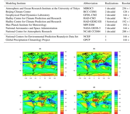
Near-surface air temperature values for 1981–2010 are taken from the NCEP/NCAR reanalysis data, provided by the Earth System Research Laboratory in the National Oceanic and At-mospheric Administration (http://www.esrl.noaa.gov/psd/). This data set originated from a project where a wide va-riety of data were assimilated from multiple sources in-cluding weather stations, ships, aircraft, radar, and satellites from 1957 onward (Kalnay et al., 1996). Data since that time continue to be assimilated and quality controlled so that complete data both in space and time are reliable and readily available (Kistler et al., 2001). The data we use are
monthly averages on a 2.5◦×2.5◦resolution grid.
Tempera-tures range from−61 to 39◦C; temperature fields are shown
in the bottom half of Fig. 1 for seasonally averaged boreal summer, June–August (JJA) and boreal winter, December– February (DJF).
Figure 1.Temperature (◦C) from GFDL for (a) JJA and (b) DJF, and from NCEP for (c) JJA and (d) DJF.
(1996) claimed that reanalysis temperature data “provide an estimate of the state of the atmosphere better than would be obtained by observations alone”. Other fields, such as precip-itation, have biases induced by the models. For this reason, we used a different data source for precipitation data.
Precipitation data was taken from the GPCP (Adler et al., 2003). Satellite and station data are compiled into
a 2.5◦×2.5◦ resolution grid of observed monthly
aver-age precipitation values from 1979 through the present. Values are reported in millimeters per day but are con-verted to kilograms per square meter per second (to match units of GCM output) assuming all precipitation has a
density of 1000 kg m−3, and range from zero to a
max-imum of 5.45×10⁻⁴kg m−2s−1, which is equivalent to
47.1 mm day−1.
The temperature values and precipitation values are de-fined at slightly different grid points, so each field had to
be adjusted to reconcile them to the same 144×72 grid.
This was done by interpolating precipitation longitudinally and temperature values latitudinally. We compute 30-year seasonal averages for boreal summer (JJA) and boreal win-ter (DJF) for the years 1981–2010. Although the averaged temperature seems to be approximately Gaussian distributed, the averaged precipitation requires transformation to allevi-ate skewness (Kleiber and Nychka, 2012); we use the cube-root transformation. The transformed precipitation fields for GPCP are shown in the bottom half of Fig. 2 for JJA and DJF.
2.2 General circulation models
Output from eight GCMs were obtained from the Program in Climate Model Diagnosis and Intercomparison (PCMDI)
server (http://cmip-pcmdi.llnl.gov/cmip5/), which archives the experimental results of the CMIP5 project. Specifically, near-surface air temperature and precipitation from 30-year decadal predictions were used (Meehl et al., 2009). The names, abbreviations and spatial resolutions of these models, all part of the CMIP5 project, are summarized in Table 1.
The data from these runs were used to compute 30-year seasonal averages for boreal summer (JJA) and boreal winter (DJF), again, for the years 1981–2010. Decadal runs were not available for HAD-GEM2-ES, the high-resolution Hadley Centre Earth Systems model, so data from part of one histor-ical run was used, specifhistor-ically December 1972–August 2003. All precipitation values were cube-root transformed. The seasonal average temperature fields from one GCM, that of the Geophysical Fluid Dynamics Laboratory (GFDL), are shown in the top half of Fig. 1, and the transformed seasonal average precipitation fields for this same GCM are shown in the top half of Fig. 2. Comparisons of GFDL fields to those of the observation proxies (NCEP/GPCP) in Figs. 1 and 2 show excellent agreement for both fields, though the details of the distributions for precipitation are not as good as for temper-ature, particularly in the extremes (JJA for the Amazon and both JJA and DJF for the Sahara and Southeast Asia).
3 Statistical method
Table 1.Names of modeling institutes and sources for observational proxy-data data.
Modeling Institute Abbreviation Realizations Resolution
Atmosphere and Ocean Research Institute at the University of Tokyo MIROC5 1 decadal 256×128
Beijing Climate Center BCC-CSM1 2 decadal 128×64
Geophysical Fluid Dynamics Laboratory GFDL-CM2 2 decadal 144×90
Hadley Centre for Climate Prediction and Research HAD-CM3 3 decadal 96×73
Hadley Centre for Climate Prediction and Research HAD-GEM2-ES 1 historical 192×195
Max Planck Institute for Meteorology MPI ESM 2 decadal 192×96
National Aeronautics and Space Administration NASA GEOS-5 2 decadal 144×91
National Center for Atmospheric Research NCAR CCSM4 1 decadal 288×192
National Centers for Environmental Prediction Reanalysis Data Set NCEP 1 144×72
Global Precipitation Climatology Project GPCP 1 144×72
Figure 2.1000 (precipitation)1/3from GFDL for (a) JJA and (b) DJF, and from GPCP for (c) JJA and (d) DJF. Precipitation values are in kilograms per square meter per second.
ALA
WNA CNAENA
GRL
NEU NAS
MED CAS TIB EAS
SEA SAH
WAF EAF
SAF CAM
AMZ
SSA AUS
SAS
ZSP ZEP ZNP
ZEA ZAE ZAN
ZNA
ZSA
ZEI
ZSI
Figure 3.Region definitions (Giorgi and Francisco, 2000).
isotropic covariance structure implies that the covariance tween two spatial locations only depends on the distance be-tween the two locations (see Sect. 3.2 for more formal defi-nition).
summa-Table 2.Climate region definitions.
Name Zone Longitude Latitude Width×height (km) 1 ALA North 180–255 60–70 3311×1113 2 WNA Mid-N 230–255 30–60 1894×3340 3 CNA Mid-N 255–275 30–50 1676×2226 4 ENA Mid-N 275–290 25–50 1292×2783 5 GRL North 255–350 60–85 2818×2783 6 NEU North 350–40 50–75 2554×2783 7 NAS North 40–180 50–70 6224×2226 8 MED Mid-N 350–40 30–50 4145×2226 9 CAS Mid-N 40–75 30–50 2921×2226 10 TIB Mid-N 75–100 30–50 2093×2226 11 EAS Mid-N 100–145 20–50 3932×3340 12 SEA Equat 95–160 −10–20 6932×3340 13 SAH Mid-N 340–65 15–30 8521×1670 14 WAF Equat 340–20 −12–15 4323×3006 15 EAF Equat 20–50 −12–15 3244×3006 16 SAF Mid-S 12–50 −35–12 3789×2560 17 CAM Mid-N 245–280 8–31 3591×2560 18 AMZ Equat 280–325 −22–8 4793×3340 19 SSA Mid-S 285–310 −54–22 2102×3562 20 AUS Mid-S 115–155 −40–16 3822×2672 21 SAS Equat 65–95 5–30 3105×2783 22 ZSP Mid-S 179–278 −40–13 9288×3006 23 ZEP Equat 179–265 −12–12 9316×2672 24 ZNP Mid-N 149–234 13–40 8053×3006 25 ZEA Equat 325–10 −20–0 4851×2226 26 ZAE Equat 310–340 0–20 3237×2226 27 ZAN Mid-N 300–340 20–40 3778×2226 28 ZNA Mid-N 310–350 40–60 2787×2226 29 ZSA Mid-S 320–10 −50–20 4360×3340 30 ZEI Equat 50–100 −20–10 5343×3340 31 ZSI Mid-S 50–110 −50–20 5207×3340
rized in Table 2. The ocean regions were only included in the exploratory data analysis phase to check our method.
3.1 Mean filtering
Before modeling the spatial dependence structure of the two climate variables, we first filter the mean structure of each of the two fields, temperature and cube-root transformed pcipitation, for each region separately, using simple linear re-gression. We write,
T =α0+α1Y+α2E+ZT,
P1/3=β0+β1Y+β2E+ZP, (1)
where Y is latitude and E elevation. We assume that the
residuals are normally distributed with mean of zero. To choose the appropriate mean structure, in addition to Eq. (1), we considered a variety of predictors, specifically
longitude X, as well as quadratic interaction terms such as
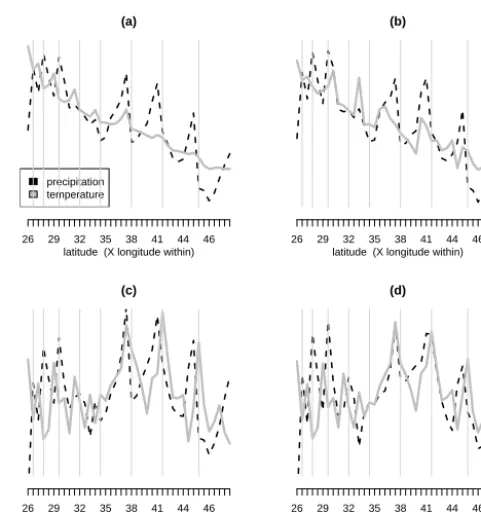
XY, XE, Y E, X2, Y2,etc. Figure 4 shows the residuals for
four different regression models for cube-root precipitation (dashed black line) and temperature (solid gray line) for the
(a)
latitude (X longitude within)
residuals
precipitation temperature
26 29 32 35 38 41 44 46
(b)
latitude (X longitude within)
residuals
26 29 32 35 38 41 44 46
(c)
latitude (X longitude within)
residuals
26 29 32 35 38 41 44 46
(d)
latitude (X longitude within)
residuals
26 29 32 35 38 41 44 46
Figure 4. Residuals after mean filtering from observational proxy data (DJF), in eastern North America (ENA): (a) Y ∼1,
(b)Y ∼elev, (c)Y∼elev+lat, and (d)Y∼elev+lat+lon.
eastern North America (ENA) region in boreal winter (DJF) for the observational proxy data. The abscissa is the index, which is arranged in scan order from the western to eastern boundaries of the region. Vertical lines denote indices where
the latitude jumps +2.5◦ and longitude jumps back to the
west boundary for a new scan back to the east. The increas-ing width between vertical bars is due to the triangular shape of ENA. As a result, the latitude dependence can be seen grossly across the graph, while longitude dependence ap-pears within each subsection. Clearly both temperature and precipitation decrease with latitude and, at least for south-ern strips, temperature rises with longitude (between vertical lines). Toward the north end of this region, positive temper-ature excursions are larger from west to east. These figures imply that a simple mean subtraction as in Eq. (1), without
higher-order terms ofX,Y, andE, is inadequate. Physically
it makes sense to subtract the linear elevation (lapse rate) and latitude dependence (solar flux), leaving the relevant second-order structure for the covariance estimation procedure. We checked figures similar to Fig. 4 for all regions for both ob-servational proxy data and GCMs and, generally, regardless of which mean structure regression was used for filtering, beyond that chosen Eq. (1), the remaining signals show very similar second-order structure.
Figure 5 shows the results of the mean field filtering process. Each plot is a specific coefficient from Eq. (1),
5 10 15 20
280
300
320
340
(a)
1:21
5 10 15 20
280
300
320
340
360
(b)
1:21
coefs[k, j, f
, 1:21, ic
, 1]
NCEP/GPCP BCC GEOS GEMS GFDL
HAD MIROC MPI NCAR
5 10 15 20
−1.0
−0.5
0.0
0.5
1.0
(e)
1:21
5 10 15 20
−2.0
−1.0
0.0
0.5
1.0
(f)
1:21
coefs[k, j, f
, 1:21, ic
, 1]
5 10 15 20
−0.010
−0.004
0.000
0.004
(i)
5 10 15 20
−0.010
−0.005
0.000
0.005
(j)
coefs[k, j, f
, 1:21, ic
, 1]
5 10 15 20
−0.06
−0.02
0.02
0.06
(c)
1:21
5 10 15 20
−0.04
0.00
0.04
0.08
(d)
1:21
coefs[k, j, f
, 1:21, ic
, 1]
NCEP/GPCP BCC GEOS GEMS GFDL
HAD MIROC MPI NCAR
5 10 15 20
−0.002
0.000
0.001
0.002
(g)
1:21
5 10 15 20
−0.003
−0.001
0.001
(h)
1:21
coefs[k, j, f
, 1:21, ic
, 1]
5 10 15 20
−1.5e−05
0.0e+00
1.0e−05
(k)
5 10 15 20
−1e−05
0e+00
1e−05
(l)
coefs[k, j, f
, 1:21, ic
, 1]
Figure 5.Mean filtering coefficients by region number (land regions only) for temperature intercept (a) JJA and (b) DJF, precipitation intercept (c) JJA and (d) DJF. Temperature latitude coefficient (e) JJA and (f) DJF, and precipitation latitude coefficient (g) JJA and (h) DJF. Temperature elevation coefficient (i) JJA and (j) DJF, and precipitation elevation coefficient (k) JJA and (l) DJF. Plots include results from NCEP/GPCP plus all eight GCMs as separate lines.
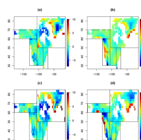
Figure 6. North America and Greenland JJA residuals: GFDL for (a) temperature and (b) 1000 (precipitation)1/3, and from NCEP/GPCP for (c) temperature and (d) 1000 (precipitation)1/3.
The abscissa is the region number (1=ALA, . . .,
21=SSA). The elevation coefficients have the least
agree-ment of the three coefficients, but generally agree well be-tween NCEP/GPCP and GCMs. Note that only land regions are included in this analysis, principally because the goal of this study is to look at those regions defined in the Giorgi and Francisco (2000) study.
Figures 6 and 7 show the residual fields for five regions: Alaska, western, central, and eastern North America, plus Greenland. The black lines in these figures delineate the boundaries of these five regions. Figure 6 shows boreal sum-mer (JJA) values while Fig. 7 shows boreal winter (DJF) val-ues. Figure 6a and b show the residual temperature and pre-cipitation fields for GFDL, while Fig. 6c and d show those for observation proxies (NCEP/NCAR-GPCP). GFDL was chosen for this example because it has the same spatial reso-lution as the observation proxies. The other GCMs have very similar residual plots.
3.2 Covariance model
We denote bivariate data consisting of the residuals from
Eq. (1) at locationsas Z(s)=(ZT(s), ZP(s)). Such bivariate
data are assumed to be isotropic, that is,
Cov{Zi(s+h), Zj(s)} =Mij(||s+h−s||)=Mij(h), (2)
whereh= ||. h||is the distance between the two locations,s
ands+h,andi, j=T orP. The covariance models,Mij,
are allowed to be different in each region to account for the fact that the spatial cross-dependence structure may vary over space on a large scale.
For modeling Mij we use the parsimonious bivariate
Matérn covariance structure developed in Gneiting et al. (2010). The Matérn covariance function is widely used to characterize the covariance of an isotropic spatial field
be-cause of its flexibility (Stein, 1999). For a univariate field,Z,
the Matérn covariance function can be written as
Cov{Z(s+h), Z(s)} =M(h)=σ22
1−ν
0(ν)(ah)
νKν(ah), (3)
whereKν(·) is the Bessel function of the second kind of order
νand0(·) is the standard gamma function,a >0, ν >0.
The covariance parameters are the variance,σ2,
smooth-ness,ν, and the inverse spatial scale,a, per kilometer.
Gneit-ing et al. (2010) offer a bivariate version of the function in Eq. (3) in the following way. Marginal covariance of each
field,ZT orZP, is given by the Matérn function in Eq. (3).
The cross-covariance of the two fields,ZT andZP, is
mod-eled as
Cov{ZP(s+h), ZT(s)} (4)
=ρσPσT
21−νP T
0(νP T)
(aP Th)νP TKνP T(aP Th).
Here, ρ gives the spatially co-located correlation
coeffi-cient satisfying a complex condition related toaP,aT,aP T,
νP,νT, andνP T (see Theorem 3 of Gneiting et al., 2010) to
guarantee a positive definite bivariate covariance function. A parsimonious version of the bivariate Matérn function
imposes a condition on the covariance parameters:a=aP =
aT =aP T andνP T =(νP+νT)/2. The condition on ρ
re-duces to|ρ| ≤
√
νPνT 1 2(νP+νT)
(Gneiting et al., 2010). Therefore,
the six covariance parameters to be estimated areσT2, σP2,
a, νT, νP, and ρ. We use a maximum likelihood
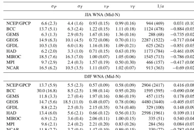
estima-tion method to estimate these parameters (refer to the Ap-pendix for details on this procedure). We compute the asymp-totic standard error for each parameter estimate, and Table 3 shows those for just one region as an example. Western North America (WNA) was chosen for this example because it is an intermediate sized region. Tables S1–S21 of the Supple-ment contain point estimates and asymptotic standard errors for all land regions for both seasons. Gneiting et al. (2010) argue that the assumption of common range parameter for the parsimonious version is not restrictive and may even be preferred due to the difficulty in estimating some of the pa-rameters in Matérn class. In our case, it is not unreasonable to assume that temperature and precipitation have similar spa-tial scales.
Co-located correlation is the spatial correlation between the precipitation and temperature fields after having been av-eraged over time, which is fundamentally distinct from the more commonly computed temporal correlation at each lo-cation (as in Trenberth and Shea, 2005, Adler et al., 2008, Tebaldi and Sansó, 2009, or Wu et al., 2013). As such, sev-eral observations are in order. First, this correlation can be computed given just one realization. Temporal correlation re-quires multiple time points to determine the extent to which the two fields correlate over time at each point in space. Sec-ond, the spatial cross-correlation coefficient can be thought of as quantifying the degree to which the residuals of the two fields share the same spatial pattern. The distinction, in terms of interpretation, is that temporal correlation tells us how the two fields compare as time unfolds for each point in space, while spatial correlation tells us how the two time-averaged fields “unfold” in space. Since we are assuming isotropic fields for each region separately, the direction separating two points is ignored, only the distance, or spatial lag, matters. We emphasize this because, while our results share features with previous studies involving temporal correlations, they also differ in important ways.
4 Results
re-Table 3.Sample region (WNA) parameter point estimate (asymptotic standard error) values.
σP σT νP νT 1/a ρ
JJA WNA (Mid-N)
NCEP/GPCP 6.6 (2.3) 4.4 (1.6) 0.93 (0.15) 0.99 (0.16) 944 (469) 0.031 (0.105) BCC 13.7 (5.1) 6.3 (2.4) 1.22 (0.15) 1.11 (0.18) 1124 (478) −0.884 (0.031) GEMS 6.3 (1.3) 2.9 (0.5) 1.67 (0.16) 1.36 (0.16) 288 (68) −0.735 (0.029) GEOS 14.9 (6.3) 10.1 (4.5) 0.72 (0.08) 0.70 (0.11) 2287 (1522) −0.717 (0.047) GFDL 10.5 (3.0) 6.0 (1.8) 1.16 (0.18) 1.09 (0.21) 625 (262) −0.851 (0.030) HAD 6.2 (2.0) 3.3 (1.0) 0.71 (0.15) 0.63 (0.19) 1173 (784) −0.461 (0.095) MIROC 18.5 (7.6) 16.3 (7.0) 1.00 (0.07) 1.05 (0.06) 1545 (713) −0.786 (0.023) MPI 9.7 (2.9) 2.4 (0.3) 1.57 (0.19) 0.50 (0.30) 466 (157) −0.417 (0.060) NCAR 16.5 (6.2) 10.5 (3.5) 1.11 (0.07) 1.02 (0.07) 913 (363) −0.69 (0.024)
DJF WNA (Mid-N)
NCEP/GPCP 13.7 (5.9) 5.5 (2.3) 0.57 (0.09) 0.58 (0.09) 2904 (2417) 0.416 (0.086) BCC 30.0 (16.8) 8.5 (2.5) 1.98 (0.14) 0.95 (0.20) 1595 (595) −0.690 (0.061) GEMS 11.8 (3.3) 2.7 (0.4) 1.97 (0.16) 0.86 (0.19) 457 (115) 0.178 (0.059) GEOS 14.7 (5.6) 18.5 (11.0) 0.48 (0.07) 0.78 (0.06) 4480 (3440) −0.405 (0.079) GFDL 8.8 (2.2) 2.5 (0.3) 2.15 (0.35) 0.74 (0.40) 329 (100) 0.148 (0.090) HAD 13.4 (6.0) 5.6 (2.1) 0.66 (0.12) 0.56 (0.13) 2598 (1961) 0.109 (0.117) MIROC 6.9 (1.2) 3.6 (0.4) 2.06 (0.11) 1.00 (0.15) 335 (51) 0.540 (0.041) MPI 9.6 (2.1) 2.4 (0.2) 2.21 (0.20) 0.83 (0.26) 284 (56) 0.084 (0.075) NCAR 11.8 (2.7) 3.7 (0.4) 1.47 (0.10) 0.89 (0.15) 330 (77) −0.282 (0.040)
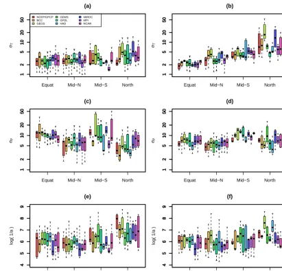
duce clutter. Typically 2–6 % of the point estimates are iden-tified as outliers, and they appear for each of the six parame-ters. There are more outliers in Equatorial and Mid-North lat-itude bands than Mid-South, and North bands because there are more Mid-North and Equatorial regions. All box plots in-clude only point estimates for land regions aggregated across latitude bands and sources (either NCEP/GPCP alone or all eight GCMs). Note that oceans are not included in the aggre-gated data. For Figs. 9 and 10, the variation within each box is due to the number of regions within a particular latitude band (5, 9, 3, and 4 points for Equatorial, Mid-N, Mid-S, and North, respectively). For Fig. 8, the dark gray NCEP/GPCP box contains this same variation, but the light gray box con-tains the variation over all eight GCMs and regions (40, 72, 24, and 32 points for Equatorial, Mid-N, Mid-S, and North, respectively).
4.1 Temperature variance,σ2 T
Figure 8a and b show the estimates ofσT versus latitude band
for observational proxy data (NCEP/GPCP) and GCMs over land only.
Note that box plots for σT have a logarithmic ordinate
axis. The pattern of both observed and modeled values shows the recognized pattern that there is very little temperature variation in the tropics throughout the year and for any lati-tude during the summer months, whereas there is much more temperature variation for mid-latitude and high-latitude loca-tions during the winter months compared to summer months
due to mid- to high-latitude storms (G. R. North, personal communication, 2014). This pattern is appropriately reversed for mid-latitude Southern Hemisphere regions (SAF, SSA, AUS), which show larger variance in summer (DJF) than winter (JJA) for both reanalysis data and GCMs.
Figure 9a and b give the estimates of σT versus
lati-tude band for reanalysis data (in red) and each GCM sep-arately. The variation within each box is due to the multi-ple regions within a latitude band and multimulti-ple realizations within GCMs. Note that for most models, the variance in-creases with latitude during winter, but not nearly as much
during the summer. The distribution ofσT values for GEOS
and MIROC, especially during boreal winter, are much more spread than other models. Equatorial regions consistently give smaller variance during DJF than JJA. Generally, the GCM models tend to overestimate the variability somewhat, particularly for high-latitude JJA.
4.2 Precipitation variance,σ2 P
Figure 8c and d show the estimates ofσP for observations,
Equat Mid−N Mid−S North 1 2 5 10 20 (a)
σT σT
1 2 5 10 20 NCEP/GPCP Models
Equat Mid−N Mid−S North
1 2 5 10 20 (b)
σT σT
1
2
5
10
20
Equat Mid−N Mid−S North
0 5 10 15 20 (c)
σP σP
0
5
10
15
20
Equat Mid−N Mid−S North
0 5 10 15 20 (d)
σP σP
0
5
10
15
20
Equat Mid−N Mid−S North
0 1 2 3 4 5 (e)
νT νT
0 1 2 3 4 5
Equat Mid−N Mid−S North
0 1 2 3 4 5 (f)
νT νT
0 1 2 3 4 5
Equat Mid−N Mid−S North
0 1 2 3 4 5 (g)
νP νP
0 1 2 3 4 5
Equat Mid−N Mid−S North
0 1 2 3 4 5 (h)
νP νP
0 1 2 3 4 5
Equat Mid−N Mid−S North
−1.0 −0.5 0.0 0.5 1.0 (i) ρ ρ −1.0 −0.5 0.0 0.5 1.0
Equat Mid−N Mid−S North
−1.0 −0.5 0.0 0.5 1.0 (j) ρ ρ −1.0 −0.5 0.0 0.5 1.0
Equat Mid−N Mid−S North
4 5 6 7 8 9 (k)
log( 1/a [km] ) log( 1/a [km] )
4 5 6 7 8 9
Equat Mid−N Mid−S North
4 5 6 7 8 9 (l)
log( 1/a [km] ) log( 1/a [km] )
4 5 6 7 8 9
Figure 8.Parameter estimates for observational proxy data and GCMs for each season by latitude band. (a) JJA and (b) DJF forσˆT, (c) JJA
and (d) DJF forσˆP, (e) JJA and (f) DJF forνˆT, (g) JJA and (h) DJF forνˆP, (i) JJA and (j) DJF forρˆ, and (k) JJA and (l) DJF for 1/aˆ(in log
scale).
they show nearly as much variance as equatorial JJA. GCMs and GPCP data differ more for Mid-S regions than other lat-itude bands for both JJA and DJF, suggesting that GCMs dif-fer from one another more in mid-latitude southern land areas than in northern and equatorial land regions.
For Mid-S JJA and North DJF, GCMs underestimate pre-cipitation variance, consistent with Zhang et al. (2007), but models overestimate variance for DJF Equat, Mid-N, and Mid-S, with all other combinations essentially equal. In all cases except Mid-S, the spread of parameter estimates over-lap well.
To explore precipitation variance for individual institute’s
GCMs, Fig. 9c and d show the estimates of σP for GPCP
data, (in red) and each institute’s GCMs separately by lat-itude band. This shows the same patterns as Fig. 8c and d. Again, the largest discrepancies are for Mid-S summer
(DJF), where all of the models except HAD and MPI over-estimate the precipitation variance, and Mid-S winter (JJA), where BCC, HAD, and MPI underestimate, while MIROC and possibly GEOS and NCAR overestimate the precipita-tion variance.
4.3 Temperature smoothness,νT
be-Equat Mid−N Mid−S North 1 2 5 10 20 50 (a) Latitude Band σT 1 2 5 10 20 50 1 2 5 10 20 50 1 2 5 10 20 50 1 2 5 10 20 50 1 2 5 10 20 50 1 2 5 10 20 50 1 2 5 10 20 50 1 2 5 10 20 50 1 2 5 10 20 50 NCEP/GPCP BCC GEOS GEMS GFDL HAD MIROC MPI NCAR
Equat Mid−N Mid−S North
1 2 5 10 20 50 (b) Latitude Band σT 1 2 5 10 20 50 1 2 5 10 20 50 1 2 5 10 20 50 1 2 5 10 20 50 1 2 5 10 20 50 1 2 5 10 20 50 1 2 5 10 20 50 1 2 5 10 20 50 1 2 5 10 20 50
Equat Mid−N Mid−S North
1 2 5 10 20 50 (c) Latitude Band σP 1 2 5 10 20 50 1 2 5 10 20 50 1 2 5 10 20 50 1 2 5 10 20 50 1 2 5 10 20 50 1 2 5 10 20 50 1 2 5 10 20 50 1 2 5 10 20 50 1 2 5 10 20 50
Equat Mid−N Mid−S North
1 2 5 10 20 50 (d) Latitude Band σP 1 2 5 10 20 50 1 2 5 10 20 50 1 2 5 10 20 50 1 2 5 10 20 50 1 2 5 10 20 50 1 2 5 10 20 50 1 2 5 10 20 50 1 2 5 10 20 50 1 2 5 10 20 50
Equat Mid−N Mid−S North
4 5 6 7 8 9 (e)
log( 1/a )
4 5 6 7 8 9 4 5 6 7 8 9 4 5 6 7 8 9 4 5 6 7 8 9 4 5 6 7 8 9 4 5 6 7 8 9 4 5 6 7 8 9 4 5 6 7 8 9 4 5 6 7 8 9
Equat Mid−N Mid−S North
4 5 6 7 8 9 (f)
log( 1/a )
4 5 6 7 8 9 4 5 6 7 8 9 4 5 6 7 8 9 4 5 6 7 8 9 4 5 6 7 8 9 4 5 6 7 8 9 4 5 6 7 8 9 4 5 6 7 8 9 4 5 6 7 8 9
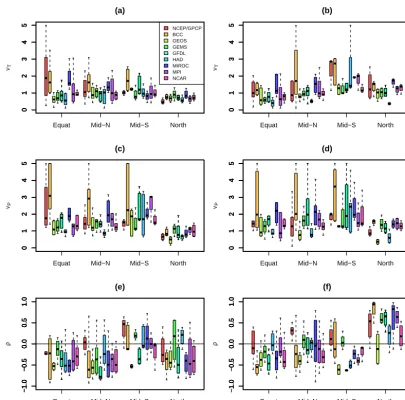
Figure 9.Parameter estimates by source for each season by latitude band, for JJA (left column) and DJF (right column). (a) JJA and (b) DJF forσˆT, (c) JJA and (d) DJF forσˆP, and (e) JJA and (f) DJF for 1/aˆ(in log scale).
tween the fields. Figure 8e and f show reanalysis data sub-stantially smoother in the tropics in JJA and southern sum-mer mid-latitudes (Mid-S DJF). Figure 10a and b show indi-vidual GCM values by region and season. BCC and MIROC tend to have the smoothest fields, while GEOS and HAD the roughest fields.
Because each GCM is evaluated at its native resolution (Table 1), we tested the dependence of this smoothness es-timate on the grid resolution. We tested for, and failed to see, association between temperature smoothness and the resolu-tion of the GCM. Large smoothness values occur for coarse models such as BCC as well as fine-gridded models such as MIROC, and vice versa. An additional test was run
us-ing GEMS at its full resolution, 288×192, versus the same
model at one-quarter its native resolution, 144×96, with little
change in final parameter estimates for most cases.
4.4 Precipitation smoothness,νP
The estimates for the smoothness parameter of the precipi-tation field in Fig. 8g and h show excellent agreement be-tween GPCP and GCMs, with roughness generally increas-ing with latitude. Figure 10c and d show the same trends by individual model. BCC has much more variation and gen-erally smoother fields, while GEOS and HAD show smaller smoothness coefficients. Again, as for temperature smooth-ness, grid resolution does not seem to be associated with pre-cipitation smoothness.
Equat Mid−N Mid−S North 0 1 2 3 4 5 (a) Latitude Band νT 0 1 2 3 4 5 0 1 2 3 4 5 0 1 2 3 4 5 0 1 2 3 4 5 0 1 2 3 4 5 0 1 2 3 4 5 0 1 2 3 4 5 0 1 2 3 4 5 0 1 2 3 4 5 NCEP/GPCP BCC GEOS GEMS GFDL HAD MIROC MPI NCAR
Equat Mid−N Mid−S North
0 1 2 3 4 5 (b) Latitude Band νT 0 1 2 3 4 5 0 1 2 3 4 5 0 1 2 3 4 5 0 1 2 3 4 5 0 1 2 3 4 5 0 1 2 3 4 5 0 1 2 3 4 5 0 1 2 3 4 5 0 1 2 3 4 5
Equat Mid−N Mid−S North
0 1 2 3 4 5 (c) Latitude Band νP 0 1 2 3 4 5 0 1 2 3 4 5 0 1 2 3 4 5 0 1 2 3 4 5 0 1 2 3 4 5 0 1 2 3 4 5 0 1 2 3 4 5 0 1 2 3 4 5 0 1 2 3 4 5
Equat Mid−N Mid−S North
0 1 2 3 4 5 (d) Latitude Band νP 0 1 2 3 4 5 0 1 2 3 4 5 0 1 2 3 4 5 0 1 2 3 4 5 0 1 2 3 4 5 0 1 2 3 4 5 0 1 2 3 4 5 0 1 2 3 4 5 0 1 2 3 4 5
Equat Mid−N Mid−S North
−1.0 −0.5 0.0 0.5 1.0 (e) ρ −1.0 −0.5 0.0 0.5 1.0 −1.0 −0.5 0.0 0.5 1.0 −1.0 −0.5 0.0 0.5 1.0 −1.0 −0.5 0.0 0.5 1.0 −1.0 −0.5 0.0 0.5 1.0 −1.0 −0.5 0.0 0.5 1.0 −1.0 −0.5 0.0 0.5 1.0 −1.0 −0.5 0.0 0.5 1.0 −1.0 −0.5 0.0 0.5 1.0
Equat Mid−N Mid−S North
−1.0 −0.5 0.0 0.5 1.0 (f) ρ −1.0 −0.5 0.0 0.5 1.0 −1.0 −0.5 0.0 0.5 1.0 −1.0 −0.5 0.0 0.5 1.0 −1.0 −0.5 0.0 0.5 1.0 −1.0 −0.5 0.0 0.5 1.0 −1.0 −0.5 0.0 0.5 1.0 −1.0 −0.5 0.0 0.5 1.0 −1.0 −0.5 0.0 0.5 1.0 −1.0 −0.5 0.0 0.5 1.0
Figure 10.Parameter estimates by source for each season by latitude band, for JJA (left column) and DJF (right column). (a) JJA and (b) DJF forνˆT, (c) JJA and (d) DJF forνˆP, and (e) JJA and (f) DJF forρˆ.
and DJF. Both coefficients are probably biased upward some-what, a conclusion based on a simulation study of the parsi-monious bivariate Matérn model (Apanasovich et al., 2012). Where we fix the spatial scale and allow both smoothness co-efficients to be fitted, Kleiber and Nychka (2012) fixed both temperature smoothness and precipitation smoothness values to 2.0, consistent with the range of values estimated here. However, the specific values are not our principle interest, but rather the comparison between estimates for GCMs and those for observational proxies. With that in mind, GCMs tend to predict less smooth fields for both temperature and precipitation in the tropics and also for southern mid-latitude summer (DJF).
4.5 Co-located cross-correlation,ρ
Estimates for the co-located cross-correlation parameter be-tween precipitation and temperature fields are given in Fig. 8i and j, and for GCM-specific plots in Fig. 10e and f. Values for proxy data and models agree very well for high-latitude regions in both seasons. Only GEOS and HAD fail to cap-ture the correct sign for this latitude band. Equatorial regions have good agreement in JJA and fair agreement for DJF. All GCMs tend to predict negative correlations over land for both seasons except high-latitude winter. Observational proxies differ most dramatically from the GCM predictions for mid-latitudes, especially during winter (DJF for Mid-N and JJA for Mid-S). Of the models considered, only a few generate positive correlations in mid-latitudes: BCC, GEMS, HAD, MIROC and, to a limited extent, GFDL and MPI.
Figure 11.Correlation coefficient maps: (a) JJA and (b) DJF for NCEP/GPCP, (c) JJA and (d) DJF for GFDL, and (e) JJA and (f) DJF for NCAR.
Fig. 11. The maps of these, plus the other six GCMs’ cor-relation estimates are shown in Figs. S1, S2, and S3 of the Supplement. Most GCMs agree with proxy data for both JJA and DJF for Alaska (ALA), northern Europe (NEU), north-ern Asia (NAS), Southeast Asia (SEA), Sahara (SAH), Aus-tralia (AUS), and India (SAS). The Mediterranean (MED), Caspian (CAS), and Amazon (AMZ) agree only for JJA, but not DJF. The remaining regions, including ocean regions, do not match well between models and observational proxies.
The values for the maps in Fig. 11 may be visualized by comparing temperature residuals and precipitation residuals from pairs of maps from Fig. 6 or 7. Consider, for exam-ple, the Greenland region (GRL) for GFDL DJF, Fig. 11d,
appear negatively correlated. The net result is a small nega-tive spatial cross-correlation for this region, indicated by the negative (blue) region in Fig. 11b. These values are tabulated in Table S5.
4.6 Correlation length,1/a
Finally, the estimated correlation length, which is con-strained to be the same for both fields’ covariance as well as the cross-covariance function, ranges from about 200 to 2000 km (see Figs. 8k and l and 9e and f), which is some-what smaller than North et al. (2011) reports, but comparable to values from Jun (2011).
5 Discussion
We present an approach for statistical models of the joint distribution of temperature and precipitation accounting for spatial dependence structure. Using a parsimonious bivariate covariance model, we compute spatial coefficients describing variation and smoothness for each field individually, as well as spatial scale and co-located correlation between the fields. Our results generally agree with previous work with sev-eral notable exceptions. Temperature variance increases with latitude in boreal winter while remaining small in summer; GCMs track these well, though with some tendency to over-estimate the variance of reanalysis data. Precipitation vari-ance decreases with increasing latitude and GCMs match ob-served values well except for southern mid-latitudes. For DJF GPCP data, precipitation variance seems to increase slightly with latitude, but decreases with latitude for GCMs. It is not clear for any latitude band or season that GCMs consistently underestimate or overestimate this variance. Smoothness es-timates for temperature fields tend to be smaller than cor-responding smoothness estimates for precipitation, and both tend to decrease with increasing latitude. Observational prox-ies, particularly in the tropics, tend to have a wider range, and smoother fields, than GCMs. Smoothness estimates for precipitation are almost entirely larger than those for temper-ature, both for proxies and all models collectively. For high latitudes, GCMs are collectively estimated to have about the same smoothness for precipitation and temperature. Overall, GCMs tend to predict smoothness coefficients near those pre-dicted by observation proxies except in the tropics, where GCMs tend to predict less smooth fields for both tempera-ture and precipitation.
Co-located cross-correlations from GCMs largely agree among models but differ from estimates from observation proxies in many regions, particularly in equatorial and mid-latitude zones. Temporal correlations are sensitive to any mean, seasonal variation, or trend that may not have been fully removed and, to some extent, this is true for spatial cor-relation estimates, though we have worked hard to minimize this. Since the aim of this study is to validate GCMs against observational proxy data, having the “right” mean structure model is not the dominant concern, but rather the consistent application across all GCMs and proxy data. Given this per-spective, it is clear that GCMs are not fully consistent with one another or with proxies, except for a few regions. Ex-ploration of this aspect of this modeling effort deserves addi-tional attention, as well as a more complete treatment of all ocean regions.
To improve the latitudinal resolution and minimize the ef-fects of specific mean structure filters, it may be possible to redefine spatial regions to smaller, more geographically ap-propriate areas, but only as GCM model resolution grows. Using some form of non-stationary covariance formulation would be a more elegant way than regional “chunking” to address this problem.
Several parameter estimates for equatorial zones show
dif-ferences between JJA and DJF, notablyσTandσP, but also
the smoothness coefficients,νT, νP, and possibly the
cross-correlation, ρ. While this may be due to noise, we think
that because there are significant annual cycles in the trop-ics (Xie, 1994; DeWitt and Schneider, 2010; Yu et al., 2013) and the fact that we consider land-only regions, it seems likely that annual temperature and precipitation effects may arise. We are not aware of any work specifically on land-only equatorial-region annual cycle effects, but our statistical method identifies these.
Appendix A: Details on maximum likelihood estimation
Once the mean structure from each field (cube-root precip-itation or temperature) is subtracted separately as done in Sect. 3.1, we assume that the residuals are a joint Gaus-sian random variable. Each variable is assumed to have
a zero mean. Let {s1, . . .,sn} denote the location of grid
points on a particular local region. Then, we have Z=
(ZT,ZP)∼N2n(0, 6(θ)), with Zj=(Zj(s1), . . ., Zj(sn)),
j =T or P, 6, a2n×2n covariance matrix, and θ=
(σT, σP, a, νT, νP, ρ) the vector of covariance parameters.
Here,Np denotes thep dimensional multivariate Gaussian
random variable.
6=
6T T 6T P
6T PT 6P P
, (A1)
where elements of6T T and6P P are given by Eq. (3) and
those of6T P are given by Eq. (4).
The log-likelihood function,
log(L(θ))= −2n
2 log(2π)−
1
2det(6(θ))−Z6
−1(θ)ZT, (A2)
is maximized at θ, which gives the estimates for the pa-ˆ
rameters. Practically, the negative log-likelihood function
is minimized numerically using the R function optim()
(R Core Team, http://www.R-project.org/). To automate this process, simulated annealing was used to explore the param-eter space, followed by the quasi-Newton algorithm Nelder– Mead, which computes the Hessian matrix, from which asymptotic errors were computed for each parameter esti-mate.
In general, the Hessian matrix is defined as
Hi,j =
∂2L(θ)
∂θi∂θj
(A3)
and the Fisher information matrix,
I(θ)i,j= −EHi,j, (A4)
which, when evaluated atθ, gives the asymptotic varianceˆ
ofθ,ˆ
var(θ)ˆ = [I(θˆ)]−1. (A5)
Author contributions. R. Philbin obtained data and reformatted it, developed and executed all code, prepared the manuscript and developed summaries. M. Jun designed study idea and indicated data source, provided core algorithm, consulted on technical details, read and fine-tuned drafts.
Acknowledgements. The authors thank G. North and R. Sara-vanan for their very constructive and helpful comments regarding this work. This publication is based in part on work supported by award no. KUS-C1-016-04, made by King Abdullah University of Science and Technology (KAUST). Also, Mikyoung Jun’s research was supported by NSF grant DMS-1208421. The authors acknowledge the World Climate Research Programme’s (WCRP) Working Group on Coupled Modelling (WGCM), which is re-sponsible for CMIP and thank the climate modeling groups (listed in Table 1 of this paper) for producing and making their model output available, as well as the WGCM for organizing the model data analysis activity. For CMIP, the US Department of Energy’s Program for Climate Model Diagnosis and Intercomparison (PCMDI) provides coordinating support and led the development of software infrastructure in partnership with the Global Orga-nization for Earth System Science Portals. The WCRP CMIP5 multi-model data set is supported by the Office of Science, US Department of Energy. The authors also acknowledge the Physical Sciences Division of the Earth System Research Laboratory in the National Oceanic and Atmospheric Administration in Boul-der, Colorado, for providing both the NCEP/NCAR Reanalysis and GPCP data from their website at http://www.esrl.noaa.gov/psd/.
Edited by: D. Cooley
Reviewed by: two anonymous referees
References
Adler, R., Huffman, G., Chang, A., Ferraro, R., Xie, P., Janowiak, J., Rudolf, B., Schneider, U., Curtis, S., Bolvin, D., Gruber, A., Susskind, J., and Arkin, P.: The Version 2 Global Precipita-tion Climatology Project (GPCP) Monthly PrecipitaPrecipita-tion Analysis (1979-Present), J. Hydrometeor., 4, 1147–1167, 2003.
Adler, R. F., Gu, G., Wang, J.-J., Huffman, G. J., Curtis, S., and Bolvin, D.: Relationships between global precipi-tation and surface temperature on interannual and longer timescales (1979–2006), J. Geophys. Res., 113, D22104, doi:10.1029/2008JD010536, 2008.
Apanasovich, T. V., Genton, M. G., and Sun, Y.: A Valid Matérn Class of Cross-Covariance Functions for Multivariate Random Fields With Any Number of Components, J. Am. Stat. Assoc., 107, 180–193, doi:10.1080/01621459.2011.643197, 2012. Christensen, J. H., Hewitson, B., Busuioc, A., Chen, A., Gao, X.,
Held, I., Jones, R., Kolli, R. K., Kwon, W.-T., Laprise, R., Rueda, V. M., Mearns, L., Menendez, C. G., Raisanen, J., Rinke, A., Sarr, A., and Whetton, P.: Climate Change 2007: Working Group I: the Physical Science Basis, chap. 11, Cambridge: Cambridge University Press, Cambridge, UK, 2007.
Colette, A., Vautard, R., and Vrac, M.: Regional climate downscal-ing with prior statistical correction of the global climate forcdownscal-ing,
Geophys. Res. Lett., 39, L13707, doi:10.1029/2012GL052258, 2012.
DeWitt, D. G. and Schneider, E. K.: Diagnosing the Annual Cycle Modes in the Tropical Atlantic Ocean Using a Directly Coupled Atmosphere–Ocean GCM, J. Climate, 20, 5319–5342, 2010. Giorgi, F. and Francisco, R.: Uncertainties in regional climate
change prediction: a regional analysis of ensemble simulations with the HADCM2 coupled AOGCM, Clim. Dynam., 16, 169– 182, 2000.
Gneiting, T., Kleiber, W., and Schlather, M.: Matérn Cross-Covariance Functions for Multivariate Random Fields, J. Am. Stat. Assoc., 105, 1167–1177, 2010.
Jun, M.: Non-stationary cross-covariance models for multivariate processes on a globe, Scand. J. Stat., 38, 726–747, 2011. Jun, M.: Matérn-based nonstationary cross-covariance models for
global processes, J. Multivar. Anal., 128, 134–146, 2014. Jun, M., Knutti, R., and Nychka, D. W.: Spatial Analysis to
Quan-tify Numerical Model Bias and Dependence: How Many Climate Models Are There?, J. Am. Stat. Assoc., 103, 934–947, 2008. Kalnay, E., Kanamitsu, M., Kistler, R., Collins, W., Deaven, D.,
Gandin, L., Iredell, M., Saha, S., White, G., Woollen, J., Zhu, Y., Chelliah, M., Ebisuzaki, W., Higgins, W., Janowiak, J., Mo, K., Ropelewski, C., Wang, J., Leetmaa, A., Reynolds, R., Jenne, R., and Joseph, D.: The NCEP/NCAR 40-year reanalysis project, B. Am. Meteorol. Soc., 77, 437–470, 1996.
Khlebnikova, E., Sall’, I., and Shkol’nik, I.: Regional climate changes as the factors of impact on the objects of construc-tion and infrastructure, Russ. Meteorol. Hydrol., 37, 735–745, doi:10.3103/S1068373912110076, 2012.
Kistler, R., Kousky, V., den Dool, H. v., Jenne, R., Fiorino, Michae-land Kalnay, E., Collins, W., Saha, S., White, G., Woollen, J., Kanamitsu, M., Chelliah, M., and Ebisuzaki, W.: The NCEP-NCAR 50-Year Reanalysis: Monthly Means CD-ROM and Doc-umentation, B. Am. Meteorol. Soc., 82, 247–267, 2001. Kleiber, W. and Nychka, D.: Nonstationary Multivariate
Spa-tial Covariance Modeling, J. Multivar. Anal., 112, 76–91, doi:10.1016/j.jmva.2012.05.011, 2012.
Lee, M., Jun, M., and Genton, M.: Validation of CMIP5 multi-model ensembles through the smoothness of climate variables, iAMCS Pre-print series 2013-385, 2013.
Li, H., Sheffield, J., and Wood, E. F.: Bias correction of monthly precipitation and temperature fields from Intergovern-mental Panel on Climate Change AR4 models using equidis-tant quantile matching, J. Geophys. Res.-Atmos., 115, D10101, doi:10.1029/2009JD012882, 2010.
Meehl, G. A., Goddard, L., Murphy, J., Stouffer, R. J., Boer, G., Danabasoglu, G., Dixon, K., Giorgetta, M. A., Greene, A. M., Hawkins, E., Hegerl, G., Karoly, D., Keenlyside, N., Kimoto, M., Kirtman, B., Navarra, A., Pulwarty, R., Smith, D., Stammer, D., and Stockdale, T.: Decadal Prediction, Can It be Skillful?, Am. Meteorol. Soc.,90, 1467–1485, doi:10.1175/2009BAMS2778.1, 2009.
North, G. R., Wang, J., and Genton, M. G.: Correlation models for temperature fields, J. Climate, 24, 5850–5862, 2011.
Sain, S. R., Furrer, R., and Cressie, N.: A Spatial Analysis of Multi-variate Output from Regional Climate Models, Ann. Appl. Stat., 5, 150–175, doi:10.1214/10-AOAS369, 2011.
Samadi, S., Wilson, C., and Moradkhani, H.: Uncertainty anal-ysis of statistical downscaling models using Hadley Cen-tre Coupled Model, Theor. Appl. Climatol. 114, 673–690, doi:10.1007/s00704-013-0844-x, 2013.
Sang, H., Jun, M., and Huang, J. Z.: Covariance approximation for large multivariate spatial datasets with an application to multiple climate model errors, Ann. Appl. Stat., 5, 2519–2548, 2011. Sargent, R. G.: Verification and validation of simulation models, J.
Simulat., 7, 12–24, doi:10.1057/jos.2012.20, 2013.
Stein, M. L.: Interpolation of Spatial Data: Some Theory for Krig-ing, Springer-Verlag New York, Inc., New York, USA, 1999. Stocker, T., Qin, D., Plattner, G., Tignor, M., Allen, S., Boschung, J.,
Nauels, A., Xia, Y., Bex, V.: IPCC, 2013: Climate Change 2013: The Physical Science Basis, Contribution of Working Group I to the Fifth Assessment Report of the Intergovernmental Panel on Climate Change, Cambridge University Press, Cambridge, UK, 2013.
Taylor, K. E., Stouffer, R. J., and Meehl, G. A.: An Overview of CMIP5 and the Experiment Design, B. Am. Meteorol. Soc., 93, 485–498, 2012.
Tebaldi, C. and Sansó, B.: Joint Projections of Temperature and Pre-cipitation Change from Multiple Climate Models: A Hierarchical Bayesian Approach, J. Roy. Statist. Soc. A, 172, 83–106, 2009.
Thorarinsdottir, T. L., Gneiting, T., and Gissibl, N.: Using Proper Divergence Functions to Evaluate Climate Models, Soc. Indust. Appl. Math., 1, 522–534, 2013.
Trenberth, K. E. and Shea, D. J.: Relationships between precipita-tion and surface temperature, Geophys. Res. Lett., 32, L14703, doi:10.1029/2005GL022760, 2005.
Wu, R., Chen, J., and Wen, Z.: Precipitation–Surface Temperature Relationship in the IPCC CMIP5 Models, Adv. Atmos. Sci., 30, 766–778, 2013.
Xie, S.-P.: On the Genesis of the Equatorial Annual Cycle, J. Cli-mate, 7, 2008–2013, 1994.
Yu, Y., He, J., Zheng, W., and Luan, Y.: Annual cycle and in-terannual variability in the tropical Pacific as simulated by three versions of FGOALS, Adv. Atmos. Sci, 30, 621–637, doi:10.1007/s00376-013-2184-2, 2013.
Zhang, F. and Georgakakos, A.: Joint variable spatial downscaling, Clim. Change, 111, 945–972, doi:10.1007/s10584-011-0167-9, 2012.