DOI 10.1186/s13408-017-0055-3
R E S E A R C H Open Access
A Rate-Reduced Neuron Model for Complex Spiking
Behavior
Koen Dijkstra1 ·Yuri A. Kuznetsov1,2·
Michel J.A.M. van Putten3,4·Stephan A. van Gils1
Received: 29 March 2017 / Accepted: 21 November 2017 /
© The Author(s) 2017. This article is distributed under the terms of the Creative Commons Attribution 4.0 International License (http://creativecommons.org/licenses/by/4.0/), which permits unrestricted use, distribution, and reproduction in any medium, provided you give appropriate credit to the original author(s) and the source, provide a link to the Creative Commons license, and indicate if changes were made.
Abstract We present a simple rate-reduced neuron model that captures a wide range
of complex, biologically plausible, and physiologically relevant spiking behavior. This includes spike-frequency adaptation, postinhibitory rebound, phasic spiking and accommodation, first-spike latency, and inhibition-induced spiking. Furthermore, the model can mimic different neuronal filter properties. It can be used to extend existing neural field models, adding more biological realism and yielding a richer dynamical structure. The model is based on a slight variation of the Rulkov map.
1 Introduction
Networks of coupled neurons quickly become analytically intractable and computa-tionally infeasible due to their large state and parameter spaces. Therefore, starting with the work of Beurle [1], a popular modeling approach has been the development of continuum models, called neural fields, that describe the average activity of large
B
K. DijkstraY.A. Kuznetsov
M.J.A.M. van Putten
S.A. van Gils
1 Department of Applied Mathematics, University of Twente, Enschede, The Netherlands 2 Department of Mathematics, Utrecht University, Utrecht, The Netherlands
3 Department of Clinical Neurophysiology, University of Twente, Enschede, The Netherlands 4 Department of Clinical Neurophysiology, Medisch Spectrum Twente, Enschede,
populations of neurons (Wilson and Cowan [2,3], Nunez [4], Amari [5,6]). In neu-ral field models, the network architecture is represented by connectivity functions and the corresponding transmission delays, while differential operators characterize synaptic dynamics. All intrinsic properties of the underlying neuronal populations are condensed into firing rate functions, which replace individual neuronal action po-tentials and map the sum of all incoming synaptic currents to an outgoing firing rate. While some neural field models incorporate spike-frequency adaptation (Pinto and Ermentrout [7,8], Coombes and Owen [9], Amari [10,11]), more complex spiking behavior such as postinhibitory rebound, phasic spiking and accommodation, first-spike latency, and inhibition-induced spiking is mostly absent, an exception being the recent reduction of the Izhikevich neuron (Nicola and Campbell [12], Visser and van Gils [13]).
Here, we present a rate-reduced model that is based on a slight modification of the Rulkov map (Rulkov [14], Rulkov et al. [15]), a phenomenological, map-based single neuron model. Similar to Izhikevich neurons (Izhikevich [16]), the Rulkov map can mimic a wide variety of biologically realistic spiking patterns, all of which are preserved by our rate formulation. The rate-reduced model can therefore be used to incorporate all the aforementioned types of spiking behavior into existing neural field models.
This paper is organized as follows. In Sect.2, we present the single spiking neuron model our rate-reduced model is based upon, and illustrate different spiking patterns and filter properties. In Sect.3we heuristically reduce the single neuron model to a rate-based formulation, and show that the rate-reduced model preserves spiking and filter properties. We give an example of a neural field that is augmented with our rate model in Sect.4and end with a discussion in Sect.5.
2 Single Spiking Neuron Model
In this section we present a phenomenological, map-based single neuron model, which is a slight modification of the Rulkov map (Rulkov [14], Rulkov et al. [15]). The Rulkov map was designed to mimic the spiking and spiking-bursting activity of many real biological neurons. It has computational advantages because the map is easier to iterate than continuous dynamical systems. Furthermore, as we will show in this paper, it is straightforward to obtain a rate-reduced version of a slightly modified version of the Rulkov model.
The Rulkov map consists of a fast variablev, resembling the neuronal membrane potential, and a slow adaptation variablea. In our modification of the original model, the adaptation only implicitly depends on the membrane potential through a binary spiking variable. As we will show in the next section, this modification allows for an easy decoupling of the membrane potential and adaptation variable, and therefore a straightforward rate reduction of the model. The cost of the modification is the loss of subthreshold oscillation dynamics. The modified Rulkov map is given by
vn+1=f (vn, vn−1, κun−an−θ ),
an+1=an−ε(an+(1−κ)un−γ sn),
where the piecewise continuous functionf: R3→Ris given by
f (x1, x2, x3)=
⎧ ⎪ ⎨ ⎪ ⎩
2500+150x1
50−x1 +50x3 ifx1<0,
50+50x3 if 0≤x1<50+50x3 ∧ x2<0,
−50 otherwise.
(1)
The form off is chosen to mimic the shape of neuronal action potentials. The vari-ableuin (SNM) represents external (synaptic) input to the cell, which we assume to be given, andsis a binary indicator variable, given by
sn=
1 if the neuron spiked at iterationn,
0 otherwise. (2)
A Rulkov neuron spikes at iterationnif its membrane potential is reset tovn+1= −50 in the next iteration. It follows from (1) that the spiking condition in (2) is satisfied if and only if
vn≥0 ∧
vn≥50+50(κun−an−θ ) ∨ vn−1≥0
. (3)
The dependence ofvn+1 onvn−1 in (SNM) ensures that a neuron always spikes if its membrane potential is non-negative for two consecutive iterations, independent of the external inputu. To mimic spiking patterns of real biological neurons, one time step should correspond to approximately 0.5 ms of time.
The parameter 0< ε <1 in (SNM) sets the time scale of the adaptation variable andγ determines the adaptation strength. The parameterθ can be interpreted as a spiking threshold: for constant external inputun=ϕ, the neuron spikes persistently
if and only ifϕ > θ. After a change of variablean→an+(1−κ)ϕ and parameter
θ→θ−ϕ, constant external input vanishes. Therefore, the asymptotic response to constant input does not depend on the parameterκ. However, the parameterκ can be used to tune the transient response of the neuron to changes in external input, as it determines how input is divided between the fast and the slow subsystem of (SNM). For parameter valuesκ ∈ [0,1],κ can be interpreted as the fraction of the input that is applied to the fast subsystem, and therefore determines (together with
ε) how quickly the membrane potential dynamics react to changes in input. Since the effective drive of the system is given byκun−an, changes in external input
are initially magnified for κ >0. Asymptotically, this is then counterbalanced by additional adaption. Finally, forκ <0, the initial response of the membrane potential to a change in input is reversed, i.e. an increase in external input initially has an inhibitory effect, and a decrease in external input initially has an excitatory effect.
2.1 Fast Dynamics
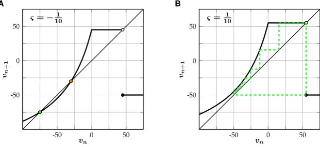
Fig. 1 Illustration of the fast subsystem (FSS) of (SNM). (A) Forς= −101 there exist a stable (green) and unstable (orange) fixed point. (B) Forς=101 the system will settle into a stable periodic orbit (dashed green line) with periodP (101)=8
an−θ=ςis constant. In this case, (SNM) reduces to the fast subsystem
vn+1=
⎧ ⎪ ⎨ ⎪ ⎩
2500+150vn
50−vn +50ς ifvn<0,
50+50ς if 0≤vn<50+50ς,
−50 otherwise.
(FSS)
The map (FSS) undergoes a saddle-node bifurcation atς=0 (Fig.1). Forς <0 there exist a stable and an unstable fixed point, given by
vs=25
ς−2− ς2−8ς, v u=25
ς−2+ ς2−8ς, (4) respectively (Fig.1A), while the system will settle into a stable periodic orbit for
ς >0 (Fig. 1B). In the former case the unstable fixed point acts as an excitation threshold: if the value of the membrane potential exceeds this point, it will spike once and then decay back to the stable equilibrium. Since the unstable fixed point
vualways lies to the right of the ‘reset potential’v= −50, a stable fixed point and a periodic orbit can never coexist. This guarantees that we can define a firing rate functionS:R→Qfor the fast subsystem (FSS), given by
S(ς )=
0 forς≤0,
1
P (ς ) forς >0,
(5)
whereP: R>0→Nmaps the drive to the period of the corresponding stable limit cycle of (FSS). The fast subsystem (FSS) is piecewise-defined on the ‘left’ interval
however, that the shape of the functionfgiven in (1) can easily be changed to support bistability in the fast subsystem, which allows for some additional dynamics such as ‘chattering’, a response of periodic bursts of spikes to constant input (Rulkov [14]).
2.2 Spiking Patterns
Izhikevich [17] classified different features of biological spiking neurons, most of which can be mimicked by our modified Rulkov model (SNM). In the following, we discuss the role of the model parameters with the help of a few physiologically relevant examples.
2.2.1 Tonic Spiking/Fast Spiking
Tonically spiking (also called ‘fast spiking’) neurons respond to a step input with spike trains of constant frequency. Most inhibitory neurons are fast spiking (Izhike-vich [17]). In the modified Rulkov model this can be achieved by choosing a ‘large’
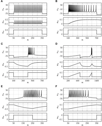
(1> ε >101)value for the time scale parameter, in which case the influence of a single spike on the adaptation variable decays very fast. Therefore, the value of the adaptation variable is dominated by the timing of the last spike and the influence of older spikes is negligible (Fig.2A). Since the time scale separation is small, the qualitative dynamics does not depend onκ.
2.2.2 Spike-Frequency Adaptation/Regular Spiking
Most cortical excitatory neurons are not ‘fast spiking’, but respond to a step input with a spike train of slowly decreasing frequency, a phenomenon known as ‘spike-frequency adaptation’ (also called ‘regular spiking’). This kind of spiking behavior can be modeled by applying all input to the fast subsystem (κ =1) and choosing
ε1. The adaptation variable then acts as a slow time scale, such that a single spike has a long-lasting effect on the adaptation variable (Fig.2B). The level of adaptation can be controlled withγ.
2.2.3 Rebound Spiking and Accommodation
The excitability of some neurons is temporarily enhanced after they are released from hyperpolarizing current, which can result in the firing of one or more ‘rebound spikes’. Rebound spiking is an important mechanism for central pattern generation for heartbeat and other motor patterns in many neuronal systems (Chik et al. [18]). In the modified Rulkov map, postinhibitory rebound spiking can be modeled by choos-ingκ >1. In this case, the adaptation variable will become negative while the cell gets hyperpolarized, which can be sufficient to trigger temporary spiking once the inhibitory input is turned off (Fig.2C). Similarly, excitatory ‘subthreshold’ (un< θ)
Fig. 2 Different types of spiking patterns generated by the single neuron model (SNM). Corresponding parameter values(θ , κ, ε, γ )are given in brackets. (A) Tonic spiking(101,21,12,12). (B) Spike-frequency
adaptation(101,1,10001 ,5). (C) Rebound spiking(501,2,1001 ,15). (D) Accommodation(253,3,501,25).
(E) Spike latency(101,0,2001 ,25). (F) Inhibition-induced spiking(501,−1,5001 ,25)
2.2.4 Spike Latency and Inhibition-Induced Spiking
in input is reversed: excitation initially leads to hyperpolarization of the neuron and inhibition can induce temporary spiking (Fig.2F). This inhibition-induced spiking is a feature of many thalamo-cortical neurons (Izhikevich [17]).
2.3 Neuronal Filtering
In the previous section, we illustrated how the parameterκcan tune transient spiking responses of the modified Rulkov map to changes in external input. In reality, neu-rons often receive strong periodic input, e.g. from a synchronous neuronal population nearby. Information transfer between neurons may be optimized by temporal filter-ing, which is especially important when the same signal transmits distinct messages (Blumhagen et al. [19]). In this section, we study the response of (SNM) to harmonic input
un=ϕcos
ωπ n
1000+ϑ
, (6)
with amplitudeϕ, phase shiftϑ∈ [0,2π ), and whereω∈ [0,1000]corresponds to the input frequency in Hz assuming that one iteration of (SNM) corresponds to 0.5 ms of time. A Rulkov neuron (SNM) will never spike if
κun−an≤θ ∀n. (7)
In this case, the adaptation reduces to the simple linear equation
an+1=(1−ε)an−ε(1−κ)un, (8)
with explicit solution
an= −ε(1−κ) ∞
m=1
(1−ε)m−1un−m. (9)
Inserting (6) into (9) now yields
κun−an=κϕcos
ωπ n
1000+ϑ
+ε(1−κ)ϕ
∞
m=1
(1−ε)m−1cos
ωπ(n−m)
1000 +ϑ
=F (ω)ϕ
2e
(1000ωπ n+ϑ )i+F (ω)ϕ
2e
−(ωπ n1000+ϑ )i
=F (ω)ϕcos
ωπ n
1000+ϑ+arg
F (ω), (10)
where the overline denotes complex conjugation and the frequency response
F: [0,1000] →Cis given by
F (ω)=κ+ ε(1−κ) e1000ωπ i +ε−1
The absolute value and argument of the frequency response determine the relative magnitude and phase of the output, respectively. It follows that a Rulkov neuron (SNM) receiving periodic input (6) does not spike if
F (ω)ϕ≤θ. (12)
The inverse statement is not true, even ifωandϑin (6) are chosen such that
cos
ωπ n
1000+ϑ+arg
F (ω)=1 for somen∈N. (13)
Since it can take a few iterations of the map to converge to its periodic orbit, a neuron will only spike if its drive is larger than the thresholdθfor a sufficiently long time. The modulus of the frequency response (11) is given by
F (ω)=
ε2+2κ(κ−ε)(1−cos(ωπ
1000))
ε2+2(1−ε)(1−cos(ωπ
1000))
, (14)
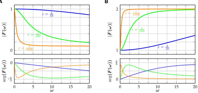
and it follows that|F|is strictly decreasing if and only ifκ ∈(−1+ε,1), and in-creasing otherwise (Fig.3). Clearly,
F (0)=1, F (1000)=2κ−ε
2−ε . (15)
The input parameterκ can therefore be used to model filter properties of the neuron. For−1+ε < κ <1 high frequencies get attenuated and a neuron can act as a low-pass filter in the sense that periodic input within a certain amplitude range only elicits a spiking response if its frequency is low enough (Fig.4A). Similarly, forκ >1 (and
κ <−1+ε), high frequencies get amplified and there exists an amplitude range for which the neuron acts as a high-pass filter (Fig.4B).
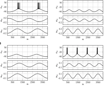
Fig. 4 Responses of (SNM) to periodic input, illustrating neuronal filter properties. (A) Forκ=101 the neuron acts as a low-pass filter. Input with an amplitude ofϕ=15 elicits a spiking response forω=1, whereas the neuron is quiescent forω=2. (B) Forκ=2, the neuron acts as a high-pass filter. Input with amplitudeϕ=101 elicits a spiking response forω=2, whereas a lower input frequency ofω=1 does not. In both examples,(θ , ε, γ )=(17,2001 ,2)
3 The Rate-Reduced Neuron Model
Neural field models are based on the assumption that neuronal populations convey all relevant information in their (average) firing rates. If one wants to incorporate certain spiking dynamics, one has to come up with a corresponding rate-reduced formulation first. In this section we present a rate-reduced version of the Rulkov model (SNM) that can be used to extend existing neural field models.
The adaptation variableain the spiking neuron model (SNM) only implicitly de-pends on the membrane potentialvvia the binary spiking variables. We can therefore decouple the adaption variable from the membrane potential by replacing the binary spiking variable defined in (2) by the instantaneous firing rate (5) of the fast subsys-tem (FSS), yielding
an+1=an−ε
an+(1−κ)un−γ S(κun−an−θ )
By interpreting (16) as the forward discretization of an ordinary differential equation, we arrive at the continuous time rate-reduced model
1
ε
da
dt = −a−(1−κ)u+γ S(κu−a−θ ). (RNM)
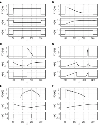
The rate-reduced neuron model (RNM) preserves the dynamical features of the full model (SNM) and reproduces all previous example spiking patterns (Fig.5).
3.1 Frequency Response of the Reduced Model
Analogously to Sect. 2.3, we now study the response of the rate-reduced model (RNM) to sinusoidal input
u(t )=ϕcos
ωπ t
1000+ϑ
. (17)
Under the assumption that
κu(t )−a(t )≤θ ∀t, (18)
the explicit solution of (RNM) is given by
a(t )= −ε(1−κ)
t
−∞e
−ε(t−τ )u(τ )
dτ, (19)
cf. (9). Inserting the input (17) into (19) yields
κu(t )−a(t )=κϕcos
ωπ t
1000+ϑ
+ε(1−κ)ϕ
t
−∞e
−ε(t−τ )cos
ωπ τ
1000+ϑ
dτ
=G(ω)ϕ
2e
(1000ωπ t+ϑ )i+G(ω)ϕ
2e
−(ωπ t 1000+ϑ )i
=G(ω)ϕcos
ωπ t
1000+ϑ+arg
G(ω),
(20) where the frequency responseG:R≥0→Cis given by
G(ω)=κ+ε(1−κ)
ε+1000ωπ i . (21)
It follows that for the rate-reduced model (RNM) receiving harmonic input (17) we have
Sκu(t )−a(t )−θ=0 ∀t if and only if G(ω)ϕ≤θ. (22) Because we neglected the transient corresponding to the convergence from fixed point to limit cycle in the rate-reduced model (RNM), the inequality in (22) defines a clear ‘spiking condition’. The modulus of the frequency response (21) is given by
G(ω)=
ε2+κ2(π ω
1000)2
ε2+(π ω
1000)2
Fig. 5 Different types of spiking behavior generated by the rate-reduced model (RNM). Top traces show the firing rate withr(t )=κu(t )−a(t )−θ. Corresponding parameter values(θ , κ, ε, γ )are given in brackets. For small values ofε (i.e. a large time scale separation), there is excellent agreement with the corresponding examples of the full model (Fig.2), which is quantified by comparing the inte-gral of the spiking rate in the reduced model to the number of spikes in the full model. (A) Tonic
spiking(101,12,12,12); 27.18(23). (B) Spike-frequency adaptation(101,1,10001 ,5); 29.13(29). (C)
Re-bound spiking(501,2,1001 ,15); 7.84(8). (D) Accommodation(253,3,501,52); 3.09(3). (E) Spike latency
and|G| therefore is strictly decreasing if and only if|κ| ≤1, and increasing other-wise. Revisiting the examples from Sect.2.3(Fig.4), we have
G(1)ϕ=0.1696. . . > θ >0.1255. . .=G(2)ϕ, (24)
for(κ, ε, θ, ϕ)=(101,2001 ,17,15), and
G(1)ϕ=0.1359. . . < θ <0.1684. . .=G(2)ϕ, (25)
for(κ, ε, θ, ϕ)=(2,2001 ,17,101). Indeed, the rate-reduced model (RNM) reproduces the examples of the full model both qualitatively and quantitatively (Fig.6). When the rate-reduced model (RNM) is incorporated into existing neural field models, the frequency response of the reduced model can be used to tune the individual temporal filter properties of the different neuronal populations.
Fig. 6 Responses of the rate-reduced model (RNM) to periodic input. Top traces show the firing rate with
r(t )=κu(t )−a(t )−θ. (A) Forκ=101 the model acts as a low-pass filter. Input with an amplitude of
ϕ=15 yields a response in the firing rate forω=1, whereas the firing rate remains zero forω=2. In the former case, the integral of the spiking rate during one period is approximately 4.55, while there are 5 spikes per period in the full model (Fig.4A). (B) Forκ=2, the reduced model acts as a high-pass filter. Input with amplitudeϕ=101 elicits a firing rate response forω=2, whereas a lower input frequency of
3.2 The Firing Rate Function
Since our neuron model (SNM) is a map, the periodP of its limit cycle lies inNfor all positive suprathreshold drivesς. Therefore, the spiking rate function (5) is staircase-like, with points of discontinuity wheneverP →P +1. Let{ς1, ς2, . . .}denote the set of all points of discontinuity of the firing rate function in decreasing order. For
ς≥ς1=1 the ‘reset potential’v= −50 in (FSS) is immediately mapped to a non-negative number, and the neuron is therefore spiking at its maximal frequency of once in three iterations. Similarly, the voltage stays in the left interval for two iterations and the neuron is spiking once in four iterations forς1> ς≥ς2=12(5−
√
17). In general, atςk, there is a jump discontinuity of size
lim
ς→ς+
k
S(ς )− lim
ς→ς−
k
S(ς )= 1
(k+2)(k+3), withS(ςk)=
1
k+2. (26)
The firing rate of the fast subsystem (FSS) can therefore be written as
S(ς )=
∞
k=1
H (ς−ςk)
(k+2)(k+3), (27)
whereH is the Heaviside step function and
lim
k→∞ςk=0. (28)
In large neuronal networks, it is often assumed that the spiking thresholds of the individual neurons are randomly distributed. This ensures heterogeneity and models intrinsic interneuronal differences or random input from outside the network. If we add Gaussian noise to the threshold parameterθin (SNM), it is natural to define an expected firing rateS:R→R, given by
S(ς )=√ 1
2π σ2
∞
−∞e
−w2
2σ2 S(ς+w)dw, (29)
whereσ2is the variance of the noise. Using (27), we can rewrite (29) as
S(ς )=1
6+
∞
k=1
erf(√ς−ςk
2σ2)
2(k+2)(k+3), (30)
where erf denotes the error function. WhileS(ς ) can readily be computed for any
ς∈Rand we derived a concise expression for the expected firing rate, the infinite sum (30) cannot easily be evaluated. For this reason, we approximateS(ς ) by a finite sum of the form
1 6+ 1 6N N
i=1 erf
ς−νi
χi
Fig. 7 Expected firing rate for a
noise level ofσ2=14. Shown are a numerical integration of (29) (blue) and its
approximation (31) forN=2 and(ν1, ν2, χ1, χ2)=(0.0335, 0.7099,0.6890,0.8213)
(orange)
for some fixedN∈Nand constantsνi, χi ∈R, which are chosen by (numerically)
minimizing
1
√
2π σ2
∞
−∞e
−w2
2σ2S(ς+w)dw−1
6− 1 6N
N
i=1 erf
ς−νi
χi
2
. (32)
For large noise levelsσ2, the average firing rate (29) has a sigmoidal shape and can be very well approximated with a small value ofN(Fig.7).
4 Augmenting Neural Fields
When large populations of neurons are modeled by networks of individual, intercon-nected cells, the high dimensionality of state and parameter spaces makes mathemat-ical analysis intractable and numermathemat-ical simulations costly. Moreover, large network simulations provide little insight into global dynamical properties. A popular mod-eling approach to circumventing the aforementioned problems is the use of neural field equations. These models aim to describe the dynamics of large neuronal popu-lations, where spikes of individual neurons are replaced by (averaged) spiking rates and space is continuous. Another advantage of neural fields is that they are often well suited to model experimental data. In brain slice preparations, spiking rates can be measured with an extracellular electrode, while intracellular recordings are much more involved. Furthermore, the most common clinical measurement techniques of the brain, electroencephalography (EEG) and functional magnetic resonance imaging (fMRI), both represent the average activity of large groups of neurons and may there-fore be better modeled by population equations. The first neural field model can be attributed to Beurle [1], however, the theory really took off with the work of Wilson and Cowan [2,3], Amari [5,6], and Nunez [4].
neurons. With the help of our rate-reduced model (RNM), it is straightforward to augment existing neural field models with more complex spiking behavior. As an ex-ample, we will look at the following two-population model on the one-dimensional spatial domainΩ=(−1,1):
1+ 1
α1
∂ ∂t
u1(t, x)=
1
−1
J11
x, xS1
r1
t, x
+J12
x, xS2
r2
t, xdx,
1+ 1
ε1
∂ ∂t
a1(t, x)= −(1−κ1)u1(t, x)+γ1S1
r1(t, x)
,
1+ 1
α2
∂ ∂t
u2(t, x)=
1
−1
J21
x, xS1
r1
t, x
+J22
x, xS2
r2
t, xdx,
1+ 1
ε2
∂ ∂t
a2(t, x)= −(1−κ2)u2(t, x)+γ2S2
r2(t, x)
,
(ANF)
where, as before,
ri(x, t )=κiui(t, x)−ai(t, x)−θi, (33)
fori∈ {1,2}. The differential operators in the left-hand side of the integral equations in (ANF) model exponentially decaying synaptic currents with decay rateαi. The
connectivityJij(x, x)measures the connection strength from neurons of population
j and positionxto neurons of populationiand positionx. The connectivity kernels
Jij:Ω×Ω→Rare assumed to be isotropic and given by
Jij
x, x=ρjηije−μij|x−x
|
, (34)
whereρj is the density of neurons of typej,ηij is the maximal connection strength,
and μij is the spatial decay rate of the connectivity. Both firing rate functions
Si: R→R are chosen to approximate the expected firing rate of Rulkov neurons
(SNM) with a noise level ofσ2=14 (Fig.7),
S1(ς )=S2(ς )= 1 6+
1 12erf
ς−0.0335 0.6890
+ 1
12erf
ς−0.7099 0.8213
. (35)
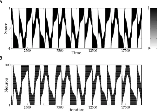
We conclude this section with a simulation of (ANF) for a particular parameter set (Table1), which illustrates that our augmented neural field can generate interest-ing spatiotemporal behavior that closely resembles spikinterest-ing patterns of a network of Rulkov neurons (SNM) with corresponding parameter values (Fig.8). In the Rulkov network, synaptic input to neuroniis given by
u(i)n+1=(1−αi)u(i)n +αi N
j=1
Fig. 8 Spatio-temporal spiking patterns. (A) Simulation of the augmented neural field (ANF) with param-eter values given in Table1. Shown is the firing rateS1(κ1u1(t, x)−a1(t, x)−θ1)of the first population.
(B) Simulation of a corresponding network of 300 excitatory and 300 inhibitory Rulkov neurons, all-to-all
coupled via simple exponential synapses. Both populations are equidistantly placed on the interval[−1,1]. Uncorrelated (in space and time) Gaussian noise with varianceσ2=14is added to the threshold parameter of each neuron. Shown is the spiking activity of the excitatory population. Each spike is denoted by a black dot
Table 1 Parameter overview for the neural field (ANF)
Parameter αi θi κi εi γi ρi ηi1 ηi2 μi1 μi2
Population 1 201 12 2 10001 5 150 23 −13 4 1
Population 2 101 45 101 1001 2 150 1115 −1130 174 1110
whereNdenotes the total number of neurons in the network, andcijis the connection
strength from neuronj to neuroni. To match the parameters in Table1, we split the total population in two subpopulations of 300 neurons each, which are both equidis-tantly placed on the interval[−1,1]. Neurons within the same subpopulation share the same intrinsic parameters, and uncorrelated (in space and time) Gaussian noise is added to the threshold parameters. Finally, the connection strengths in the Rulkov network are given by
cij=ηpipje
−μpi pj|xi−xj|, (37)
5 Discussion
This paper presents a simple rate-reduced neuron model that is based on a variation of the Rulkov map (Rulkov [14], Rulkov et al. [15]), and can be used to incorporate a variety of non-trivial spiking behavior into existing neural field models.
The modified Rulkov map (SNM) is a phenomenological, two-dimensional single neuron model. The isolated dynamics of its fast time scale either generates a stable limit cycle, mimicking spiking activity, or a stable fixed point, corresponding to a neuron at rest (Fig.1). The slow time scale of the Rulkov map acts as a dynamic spiking threshold and emulates the combined effect of slow recovery processes. The modified Rulkov map can mimic a wide variety of spiking patterns, such as spike-frequency adaptation, postinhibitory rebound, phasic spiking, spike accommodation, spike latency and inhibition-induced spiking (Fig.2). Furthermore, the model can be used to model neuronal filter properties. Depending on how external input is applied to the model, it can act as either a high-pass or low-pass filter (Figs.3and4).
The rate-reduced model (RNM) is derived heuristically and given by a simple one-dimensional differential equation. On the single cell level, the rate-reduced model closely mimics the spiking dynamics (Fig.5) and filter properties (Fig.6) of the full spiking neuron model. While a close approximation of the (expected) firing rate of Rulkov neurons (Fig.7) is needed to mimic their behavior quantitatively, the types of qualitative dynamics of the rate-reduced model do not depend on the exact choice of firing rate function.
Due to its simplicity, it is straightforward to add the rate-reduced model to existing neural field models. In the resulting augmented equations, parameters can be chosen according to the spiking behavior of a single isolated cell. In our particular example (ANF), the emerging spatiotemporal pattern closely resembles the dynamics of the corresponding spiking neural network (Fig.8). We believe that this is an elegant way to add more biological realism to existing neural field models, while simultaneously enriching their dynamical structure.
5.1 Conclusions
We used a variation of a simple toy model of a spiking neuron (Rulkov [14], Rulkov et al. [15]) to derive a corresponding rate-reduced model. While being purely phe-nomenological, the model could mimic a wide variety of biologically observed spik-ing behaviors, yieldspik-ing a simple way to incorporate complex spikspik-ing behavior into existing neural field models. Since all parameters in the resulting augmented neural field equations have a representative in the spiking neuron network (and vice versa), this greatly simplifies the otherwise often problematic translation from results ob-tained by neural field models back to biophysical properties of spiking networks. An example demonstrated that the augmented neural field equations can produce spa-tiotemporal patterns that cannot be generated with corresponding ‘classical’ neural fields.
Funding K.D. was supported by a grant from the Twente Graduate School (TGS).
Ethics approval and consent to participate Our study don’t involve human participants, human data or human tissue.
Competing interests The authors declare no competing financial interests.
Consent for publication This manuscript does not contain any individual person’s data.
Authors’ contributions Conceptualization, K.D., Y.K., M.v.P. and S.v.G.; methodology, K.D. and S.v.G.; investigation, K.D.; writing original Draft, K.D.; writing review & Editing, K.D., Y.K., M.v.P. and S.v.G.; visualization, K.D.; supervision, Y.K., M.v.P. and S.v.G. All authors read and approved the final manuscript.
Publisher’s Note
Springer Nature remains neutral with regard to jurisdictional claims in published maps and institutional affiliations.
References
1. Beurle RL. Properties of a mass of cells capable of regenerating pulses. Philos Trans R Soc Lond B. 1956;240:55–94.
2. Wilson HR, Cowan JD. Excitatory and inhibitory interactions in localized populations of model neu-rons. Biophys J. 1972;12:1–24.
3. Wilson HR, Cowan JD. A mathematical theory of the functional dynamics of cortical and thalamic nervous tissue. Kybernetik. 1973;13:55–80.
4. Nunez PL. The brain wave equation: A model for the EEG. Math Biosci. 1974;21:279–97. 5. Amari S. Homogeneous nets of neuron-like elements. Biol Cybern. 1975;17:211–20.
6. Amari S. Dynamics of pattern formation in lateral-inhibition type neural fields. Biol Cybern. 1977;27:77–87.
7. Pinto DJ, Ermentrout GB. Spatially structured activity in synaptically coupled neuronal networks: I. Traveling fronts and pulses. SIAM J Appl Math. 2001;62:206–25.
8. Pinto DJ, Ermentrout GB. Spatially structured activity in synaptically coupled neuronal networks: II. Lateral inhibition and standing pulses. SIAM J Appl Math. 2001;62:226–43.
9. Coombes S, Owen MR. Bumps, breathers, and waves in a neural network with spike frequency adap-tation. Phys Rev Lett. 2005;94:148102.
10. Kilpatrick ZP, Bressloff PC. Effects of synaptic depression and adaptation on spatiotemporal dynam-ics of an excitatory neuronal network. Physica D. 2010;239:547–60.
11. Kilpatrick ZP, Bressloff PC. Stability of bumps in piecewise smooth neural fields with nonlinear adaptation. Physica D. 2010;239:1048–60.
12. Nicola W, Campbell SA. Bifurcations of large networks of two-dimensional integrate and fire neurons. J Comput Neurosci. 2013;35:87–108.
13. Visser S, van Gils SA. Lumping Izhikevich neurons. EPJ Nonlinear Biomed Phys. 2014;2:226–43. 14. Rulkov NF. Modeling of spiking-bursting neural behavior using two-dimensional map. Phys Rev E.
2002;65:041922.
15. Rulkov NF, Tomofeev I, Bazhenov M. Oscillations in large-scale cortical networks: Map-based model. J Comput Neurosci. 2004;17:203–23.
16. Izhikevich EM. Simple model of spiking neurons. IEEE Trans Neural Netw. 2003;14:1569–72. 17. Izhikevich EM. Which model to use for cortical spiking neurons? IEEE Trans Neural Netw.
2004;15:1063–70.
18. Chik DTW, Coombes S, Wang ZD. Clustering through postinhibitory rebound in synaptically coupled neurons. Phys Rev E. 2004;70:011908.