e-ISSN: 2278-067X, p-ISSN: 2278-800X, www.ijerd.com
Volume 14, Issue 3 (March Ver. I 2018), PP.17-27
Application and Optimization of Control Implemented In
Irrigation Systems Based On Microclimate Models of Tropical
Crops
Carlos S. Cohen Manrique
1, Jhonatan A. Rodríguez Manrique
2, Guillermo C.
Hernández Hernández
31 , 2, 3 Corporación Universitaria del Caribe-CECAR, km 1 via Corozal, Sincelejo-Sucre, Colombia.
Corresponding Author: Carlos S. Cohen Manrique
ABSTRACT:-It presents a simulation study oriented to the control of irrigation systems, whose main objective was to evaluate the performance in terms of stability of controllers based on the fuzzy logic and PID, which have as a characteristic the emulation of human knowledge and traditional use in industrial applications respectively. Both control systems interacted with the different models and sub-models related to the microclimate of plants, so that their fundamental purpose was to maintain soil moisture and the water requirements of the crop. As a control strategy, it was defined as an input signal the difference between the humidity level supported by the existing soil type and the actual humidity level measured in each instant of time through electronic sensors. The water balance equation, i. e. the interaction between climate, crop and soil subsystems, was used as a strategy to model these moisture levels. These were parameterized under the climatic conditions of the study area and adapted to the different types of soils in the municipality of Sincelejo (Colombia). Finally, we propose the best control alternative that optimizes water management in irrigation systems for watermelon crops, taking as a decision criterion the stability of the system and its energy consumption. It is concluded that the irrigation model based on the PID controller achieved better performance in terms of stability, energy consumption and reliability, but the diffuse controller uses less liquid to maintain water requirements, however, the continuous intermittent operation presumably makes the controller susceptible to increased power consumption.
KEYWORDS:- Irrigation systems, fuzzy logic, PID controllers, water balance, precision agriculture.
--- Date of Submission: 22 -02-2018 Date of acceptance: 09-03 2018
---I. INTRODUCTION
The world population is growing rapidly and according to global projections mainly in the least developed countries, where the population is growing at a rate five times higher than in developed countries (FAO, 2011). This growth implies that agriculture remains the essential engine of growth for economic development and environmental services, and for reducing rural poverty. In Colombia, approximately 70% of the freshwater used for human consumption is destined for the agricultural sector (Steduto et al., 2012). This high percentage of extraction and consumption in the country is due to the demand for each of the permanent or transitory crops that are used to sustain food for people and animals (Pacheco Riaño, 2017).
In this writing, mathematical models are used to be used in the simulation of the variables involved in water consumption for a watermelon crop (Citrullus lanatus). For this purpose, consideration was given to the water balance point presented by Laio et al., (2001), where the dynamics of soil moisture losses and the effects of perspiration are modelled, which is defined as the microclimate of plants. To do this, some models such as Penman Monteith (PM) are used to evaluate evapotranspiration (Allen et al., 2006) used by Norero (1976) for estimating the daily root growth of the plant and its impact on water consumption, Liotta (2007) for the evaluation of water volumes for irrigation in watermelon crops, James (2012) for the flow balance process, Mendoza-Díaz (2009) for the soil study model in the Sincelejana Savannah, Kostiakov - Lewis for calculating the velocity (Laio et al., 2001), Lop et al., (2005) for the model for estimating useful water in plants, Flores and Ruíz (1999) for the desired humidity model in soils and Hernández-Tórres (2010) for the eco-hydrological model of punctual water balance, among others. Evaluated all of them, through dynamic modelling defined to recreate the global water requirements of the plants, as close as possible to reality and demonstrating that this is a process totally controllable in time and usable for studies oriented to agricultural production.
II. MATERIALS AND METHODS
The project used modelling and simulation tools for encapsulating the plant's microclimate, in a transfer function modelled over time, so that it could be controlled through a mathematical model (transfer function) that facilitates the adjustment of the constants of a proportional, integral and derivative controller (PID), respectively Kp, Ki and Kd. This, so that it can be implemented in an efficient and simple way, studying
its stability in terms of gain, poles and zeros using some traditional methods, such as the geometric place of the roots, tuning techniques such as Ziegler Nichols (O'Dwyer, 2006), so that the ideal tuning can be found. In parallel, the fuzzy controller was used as an important alternative due to its ease of application related to its intuitive interface and easy applicability, so that tuning was done based on rules aimed at correcting the error that occurs when comparing the input and output functions of the plant.
For this purpose, the main climatic variables of the study area were defined, using the satellite weather station of the Sucre University, located in the municipality of Sincelejo, from which a total of 17,280 data were obtained from precision sensors. These data correspond to air temperature, precipitation, global radiation, relative air humidity, atmospheric pressure, wind speed and direction, being measured with an hourly periodicity. These records fed the model of Penman Monteith Allen et al., (2006) to recreate the water consumption of the crop through the evapotranspiration process (Equation 1). The data taken and applied to the simulation study were selected from the measures corresponding to the months in which watermelon is grown in the study area, namely March, April, May and June.
2
2
37
0.408 ( ) ( )
273 (1 0.34 )
n s a
o
R G U e e
T ET U (1)
Where, ETo is the reference evapotranspiration (mm/day), Rn is the net radiation on the crop surface
(MJ/m2 day), G is the flow of soil heat (MJ/m2 day), T is the average air temperature at two meters high (°C), U 2
is the wind velocity at two meters high (m/s), es-ea is the actual vapor pressure (kPa), Δ is the slope of the steam
pressure curve (kPa/°C) and finally
is the psychrometric constant (kPa/°C). In addition to modelling evapotranspiration, the cultivation coefficient Kc and its phenological stages, the soil's water properties were modelled, worked from some mathematical models subject to the principle of conservation of mass. To model the soil zone, the water balance model was used following the methodology of Laio (2001) and Rodríguez-Iturbe and Porporato (2007), considering the porous medium as a structure of small interconnected ducts of diameter n and taking into account the laminar flow expressed by the Darcy's Law (Sanchez, 2011) in such a way that:Where, n is the soil porosity, Zr is the active depth of the root zone of the plant, s(t) is the relative
moisture content of the soil, φ[s(t);t] is the infiltration rate, χ[s(t)] is the rate of moisture loss from the root zone. The study region used for the implementation of the control system corresponds to a tropical dry forest zone and its characteristic landscape is the mountain. The predominance of fog is common in hillside forests during the early morning and evening hours. The action of trade winds during the dry season influences the regulation of temperature, relative humidity and precipitation. It has two well marked seasons, during the summer that
( )
[ ( ); ] [ ( )] r
ds t
nZ s t t s t
extends for more than eight months a year, the temperature rises and the soils are very prone to dryness and erosion. Likewise, for the winter season rainfall is continuous and copious. Figure 1, shows the behaviour of some variables on a summer day in the study area and at sowing time.
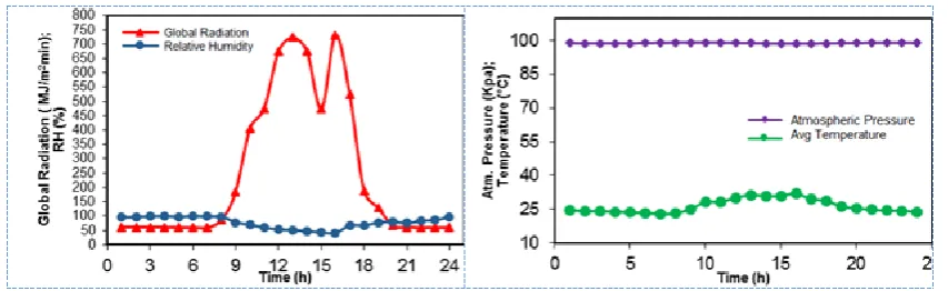
Fig. 1: Sample of global radiation, relative humidity, atmospheric pressure and average temperature in the study region (Savannahs of the department of Sucre) on one day during the watermelon harvest.
It can be inferred from Figure 1 that the radiation and temperature values are quite high averaging midday, staying well into the night. This indicates that the sun's rays hit the crops hard during a good part of the day, producing liquid requirements.
Similarly, the model (2) not only includes consumption by transpiration of the crop but also adds the soil's water activity, where some quantities of water are absorbed by the roots, others do not penetrate the soil and others are infiltrated through the soil without being useful for the plants (Moreno and Osorno 1999), and is shown in figure 2, producing the deep percolation and that in this document is not included, because of the difficulty of measurement and the low percentage contribution to the totality of liquid drained by precipitation or irrigation. The general model of the plant microclimate used for the control system is shown in Figure 3, where precipitation rate R(t) is shown, in addition to losses due to infiltration I(t), surface runoff Q[s(t);t), evapotranspiration E[s(t)] and deep percolation L[s(t)]. From equation 2, the complete model used in the control system can be inferred (Rodríguez-Iturbe, 1999; Laio et al., 2001; Porporato et al., 2004; Hernández Tórres, 2010).
( )
( ) ( ) ( ); ( ) ( ) r
ds t
nZ R t I t Q s t t E s t L s t
dt (3)
Once the models that simulated the different variables that represent the plant's microclimate (3) have been defined, the control systems are defined. Two types of controllers were used, one proportional, integral derivative (PID) and one diffuse. Both using the same input data and the same simulation model, to compare its operation and establish which one best adapts to the dynamic conditions of the microclimate presented in the Sucre Savannahs.
Fig. 2: Infiltration rate graph for soil types in the savannah of Sucre department.
First, a tuned PID Control system was used. Based on its classic configuration, using the respective gain (Kp) and tuning the design variables related to the proportional, integral and derivative controller Kp, Ki, Kd.
Fig. 3: Distribution of fluid loss in the plant (Laio et al., 2001).
When tuning the controller experimentally, as proportional, integral and derivative design parameters, the values of Kp = 2, Ki = 0.1, Kd = 0.3 were obtained respectively, so that the response delivered in terms of
actual humidity or measured with the desired humidity, produced an error of approximately 0%. This subjecting the controller to various tuning and stability tests, to establish whether the control system was following the desired signal. This is how we proceeded to change the block that models the desired humidity (system input signal) by a source with a stepped signal, then by a source with a constant signal and/or finally, a source with a ramp type signal. For all of them, the system showed total stability and an error signal response very close to zero. This could ensure that the PID controller is correctly tuned. Figure 4 shows the PID controller designed in Matlab® using its development tool Simulink®.
To control irrigation, the irrigation control system used a measure of the actual moisture level of the soil, and then compared it to the desired moisture level or moisture level supported by the soil. In general, the difference between the desired humidity level and the current humidity level is equal to the error, which is set by the controller via a feedback control loop. The controller output causes the actuator to regulate the process for the purpose of reducing error by opening or closing the valve so that the difference between the moisture level data is continuously reduced. For practical purposes, the estimation model for useful water in plants (UPA) was used as design ranges, in fact, the optimum moisture level at which the crop should remain, either because of precipitation levels or the control system's action. This UPA level is defined as the difference between the value of the field capacity (FC) and the permanent wilting point of the crop (PMP). Both models are included in the block called Water Balance of Figure 3 (Lop et al., 2005; Dukes et al., 2010; Osuna and Ramírez, 2013).
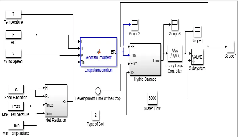
Fig. 4: Tuned PID Controller applied to the microclimate model.
of Mamdani's inference has the advantage that the areas of the belonging functions are not used, but each contribution is operated separately and a weighted average of the contribution centers is calculated, which simplifies the mathematical analysis of their behavior (Berengi, 1996). In addition, the diffuse mamdani system is the most widely used in the Fuzzy methodology (Nicolas, 2008).
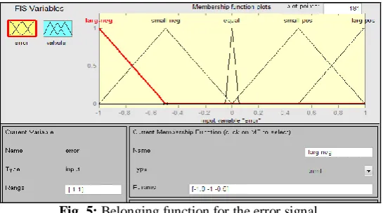
Fig. 5: Belonging function for the error signal.
Figure 5 shows the membership functions used as diffuse driver rules in the Matlab® software, which can be seen in table 1. Five language labels are assumed: Very Negative (LN), Little Negative (SN), Zero (E), Little Positive (SP) and Very Positive (LP).
Table 1. Rules used in the diffuse controller to evaluate the microclimate of the plant. Fuzzy Controller Rules
1. If the Error is Very Negative (LN), then Valve Closes Quickly 2. If the Error is Little Negative (SN), then Valve Closes Slowly. 3. If Error is Zero (E), then Valve Does Not Change
4. If the Error is Poorly Positive (SP), then Valve Open Slowly 5. If the Error is Very Positive (LP), then Valve Open Quickly
This set of fuzzy rules decided based on the error of the humidity level, the position in which the valve was adjusted. These rules were obtained by making a heuristic analysis of the possible decisions that would have been made if the operator were a human (Juárez et al., 2011).
Figure 6, illustrates the fuzzy division of the controller's output spaces with their respective language labels and their triangular function. The membership functions performed on the valve are observed, i. e. when these rules are executed on the diffuse controller the valve will open or close gradually, as the case may be. This limits the amount of water available for each irrigation terminal (gutter) according to the water requirement of the plant.
Fig. 6: Function belonged to the valve control.
Choudhary, 2011) as the basic equation. In figure 7, the diffuse controller is shown, where the feedback of the output on the valve is observed, i. e. the amount of water in the irrigation, so that the water balance block defines the current value of the differentiated humidity with the desired value.
Fig. 7: Diffuse Controller applied to the microclimate model
III. RESULTS AND DISCUSSION
The execution time of the model under consideration is the lifespan of the watermelon crop, estimated between 90 and 110 days corresponding to 3 months and 20 days, i. e. 720 hours of monthly simulation (2,640 hours in total), the latter being the units of time in which the system is executed. In order for the model simulation and controller structure to function properly, the format of the data included in each of the models was matrix at hourly intervals, some of them provided directly by the weather station, others indirectly through sub-models (Allen et al., 2006) and others through their temporal assessment due to crop growth. By practicality, daily runs of the model were carried out to know its behavior before variable input signals in time such as those of the Penman-Monteith model, the model of root size, the model that establishes water requirements, among others. All this to try to understand first-hand the performance of the controllers, the fluid consumption, the work of the valve, and so on. The graphical results are shown in the following figures.
0.0 0.2 0.4 0.6 0.8 1.0 1.2
0 2 4 6 8 10 12 14 16 18 20 22 24
M
o
is
tu
re
(m
m
)
Time (hr)
Real Moisture
Desired Moisture in the Soil
Fig. 8: Comparison of Real Humidity and Desired Soil Humidity for PID over 24 hours.
Now, for the fuzzy controller. Figure 9, shows the relationship between Desired Humidity and Actual Humidity after the controller's work.
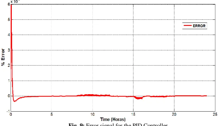
Fig. 9: Error signal for the PID Controller.
Fig. 10: Comparison between actual and desired soil moisture for the fuzzy controller.
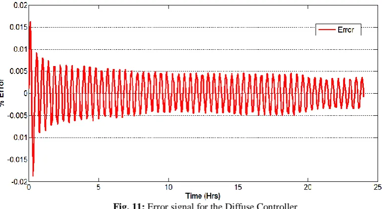
In figure 11, the error signal (difference between the desired and actual humidity) is shown at the output of the adder in the fuzzy controller, and it can be inferred that the values of the same in percentage terms exceed slightly 1.5%, which according to Rahangdale and Choudhary (2011) is a valid value for a control system, and even more so for an agricultural application where the margins of the error can be high. In addition to this, it can be said that in certain hours of the day and for relatively short periods of time the error is zero, which shows the stability of the system and the optimization of the water resource; unfortunately it is oscillating and with an approximate oscillation period of 2.4 cycles/hour, but with amplitude values almost constant of ±1.5% approximately.
Fig. 11: Error signal for the Diffuse Controller.
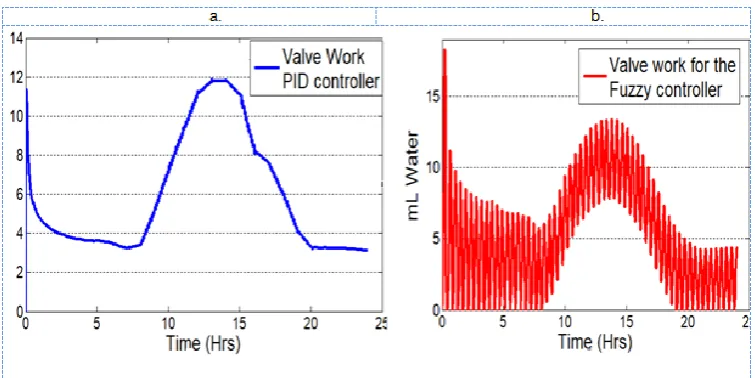
Fig. 12: Valve working signal for diffuse controllers (a) and PID (b).
The maximum amount of work carried out (amount of irrigation supplied to the crop) by the valve, when the controller is diffuse (Figure 12a), occurs approximately between 13 and 14 hours a day, with a value close to 13 milliliters (12,6755 ml), this without taking into account the initial expenditure (first hour of irrigation). In contrast to the PID controller (Figure 12b), the diffuse controller shows an alternating irrigation, i. e. irrigation is not continuous, but in long periods of time the amount of water is oscillatory, which increases ostensibly the work in the valve, but also the maximum consumption exceeds 18.29 milliliters, during the first hour of work, and on average consumption reaches 1.7533 milliliters of water.
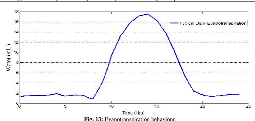
Fig. 13: Evapotranspiration behaviour.
The graphical behavior of the Penman-Monteith model (equation 1) and figure 13, responds to the typical behavior of this model in different parts of the world (Gong and Xu, 2005; Allen, 2006; Nghi, 2008; Mundo-Molina, 2008; Howell, 2010; Adeboye and Osunbitan, 2010). This demonstrates the correct application of the same one, based on the climatic parameters circumscribed to the Savannah region of the department of Sucre. On the other hand, if the value of Kc (phenological plant age) is varied, or the type of crop is changed, so
that this value of Kc represents another stage of plant growth, with other water requirements, the behavior of the
controller would be the same. An easy way to comply with the paper formatting requirements is to use this document as a template and simply type your text into it.
IV.
CONCLUSIONS
It is concluded that, under the parameters used in it, the irrigation model based on the PID controller achieved better performance in terms of stability, energy consumption and reliability, but the diffuse controller uses less liquid to maintain water requirements, despite the permanent intermittence in its operation that is presumed to make the controller susceptible to increased energy consumption. But in general terms, it has been possible to define a water model that is independent of the type of controller, proves to be controllable and dynamically manipulable. This is important when it comes to field implementation, as modelling saves a lot of money and time because some models would replace the purchase of precision sensors that are usually very expensive for the farmer. It also facilitates the implementation of it in its later implementation in other types of crops, land, types of irrigation.
REFERENCES
[1]. Adeboye, O., and J. Osunbitan, “Evaluation of FAO-56 Penman-Monteith and Temperature Based Models in Estimating Reference Evapotranspiration Using Complete and Limited Data, Application to Nigeria”. Ile-Ife, Nigeria: Department of Agricultural Engineering (2010).
[2]. Allen, R., L. Pereira, D. Raes, y M. Smith, “Evapotranspiración del Cultivo: Guías para la Determinación de los Requerimientos de Agua de los Cultivos”. Roma, Italia: FAO (2006).
[3]. Berengi, H., “Fuzzy and Neural Control”. New York, USA: Intelligent and Autonomuos Control (1996). [4]. Bitar, S., “Las tendencias mundiales y el futuro de América Latina”, (2014).
[5]. Díaz, M. “La economía del departamento de Sucre: ganadería y sector público. Banco de la República”, Centro de Estudios Económicos Regionales, (2005).
[6]. Dukes, M. D., L. Zotarelli, y K. Morgan, “Use of irrigation technologies for vegetable crops in Florida”. HortTechnology, 20(1) 133-142 (2010).
[7]. FAO. “Estado de los Recursos de Tierras y Aguas del Mundo para la Alimentación y la Agricultura”. Roma: FAO, Fiat Panis. (2011).
[8]. Flores, H., y J. Ruíz, “Estimación de la Humedad del Suelo para Maíz de Temporal Mediante un Balance Hídrico”. Jalisco, México: ANIFAP - CIPAC (1999).
[9]. Gong, L., y C. Xu, “Sensitivity of the Penman–Monteith Reference Evapotranspiration to Key Climatic Variables in the Changjiang (Yangtze River) Basin”. Basin, China: Uppsala University (2005).
[10]. Hernández Torres, G., “Modelamiento eco-hidrológico de la humedad del suelo en el valle del Río Cauca”, Tesis Doctoral, Universidad Nacional de Colombia (2010).
[11]. Howell, T. “The Penman - Monteith Method. Bushland”, USA: USDA - Agricultural Research Service. (2010).
[12]. IGAC, U. “Atlas de la distribución de la propiedad rural en Colombia”. Instituto Geográfico Agustín Codazzi, Universidad de los Andes, Bogotá (2012).
[14]. Javadi, P., M. Omid, y L. Nomb, “Intelligent Control Based Fuzzy Logic for Automation of Grrenhouse Irrigation System and Evaluation in Relation to Conventional Systems”. World Applied Sciences Journal, 16 – 23 (2009).
[15]. Juárez, J., J. Cañadas, y M. Roque, “Sistemas de Control Moderno”, Murcia, España: Universidad de Murcia, Universidad de Almería, (2011).
[16]. Klee, H., y Randal, A. “Simulation of Dynamic Systems with Matlab and Simulink”. Boca Ratón, Florida: CRC Press. (2011). [17]. Laio, F., Porporato, A., Ridolfi, L., y Rodriguez-Iturbe, I. “Plants in water-controlled ecosystems: active role in hydrologic
processes and response to water stress: II. Probabilistic soil moisture dynamics”. Advances in Water Resources, 24(7), 707-723. (2001).
[18]. Liotta, M. “Los Sistemas de Riego por Goteo o por Microasperción”. San Juan, Puerto Rico: INTA - EEA.iturb(2007).
[19]. Lop, A., C. Peiteado, y V. Bodas, “Curso de riego para agricultores. Proyecto de autogestión del agua en la agricultura de la WWF y Acciones Integradas de desarrollo”, (2005).
[20]. Mamdani, E. “An Experiment in Linguistic Synthesis with a Fuzzy Logic Controller”. New York, USA: International Journal of Man-Machine Studies (1975).
[21]. Mendoza Diaz, J. F. “Determinación de ecuaciones lineales de capacidad de campo para tres tipos de suelos arcilloso, franco arcilloso y franco, presentes en la ciudadela universitaria Puerta Roja, Sincelejo, Sucre” Tesis Doctoral, (2009).
[22]. Moreno, F., & Osorno, J. Estudio Comparativo de los Métodos de Laboratorio para la determinación de Capacidad de Campo y Obtención de Ecuaciones. Sincelejo, Sucre: Universidad de Sucre. (1999)
[23]. Mundo-Molina, M. “Estandarización de las ecuaciones para estimar la evapotranspiración del cultivo de referencia”. RIIT FI - UNAM, 125 - 135 (2008).
[24]. Nghi, V. V., “Potencial Evapotranspiration Estimation and its effect on Hydrological Model Response at the Nong Son Basin. VNU Journal of Science, 213 - 223 (2008).
[25]. Nicolás, I., “Técnicas de compresión de tablas de datos mediante regresiones lineales, redes neuronales y sistemas fuzzy”. Murcia, España: Universidad Politécnica de Cartagena (2008).
[26]. Norero, A., “Evaporación y Transpiración: Serie Suelos y Climas”. Mérida, Venezuela: CIDIAT (1976). [27]. O'Dwyer, A., “Handbook of PI and PID controller tuning rules”. World Scientific. (2009).
[28]. Osuna-Canizalez, F. D. y S. Ramírez-Rojas, “Manual para cultivar cebolla con fertirriego y riego por gravedad en el estado de Morelos”, (2013).
[29]. Pacheco Riaño, A. M., y A. Garzón Bustamante, “Formulación de estrategias de mejora de consumo de agua en la producción de Feijoa en la finca Cortijo de la Merced en la Vega–Cundinamarca”, (2017).
[30]. Perfetti, J. J., A. Hernández, J. Leibovich, y Á. Balcázar, “Políticas para el desarrollo de la agricultura en Colombia” (2013). [31]. Porporato, A., Daly, E., y I. Rodriguez-Iturbe, “Soil water balance and ecosystem response to climate change”. The American
Naturalist, 164(5), 625-632 (2004).
[32]. Rahangadale, V., y D. Choudhary, “On Fuzzy Logic Based Model for Irrigation Controller Using Penman - Monteith Equation”. Gondia, India: MIET (2011).
[33]. Rodriguez-Iturbe, I., A. Porporato, L. Ridolfi, V. Isham, y D. Coxi. “Probabilistic modelling of water balance at a point: the role of climate, soil and vegetation. In Proceedings of the Royal Society of London”, Mathematical, Physical and Engineering Sciences, 455(1990), 3789-3805 (1999).
[34]. Ruíz, V. A. “Métodos de sintonización de controladores PID que operan como reguladores”. Revista Ingeniería, 12(1-2) (2011). [35]. Sánchez San Román, J. “Ley de Darcy. Conductividad Hidráulica”. Salamanca, España: Universidad de Salamanca (2011). [36]. Steduto, P., T. C. Hsiao, E. Fereres, y D. Raes, “Respuesta del rendimiento de los cultivos al agua”. Estudio FAO: Riego y Drenaje
(FAO) spa no. 66 (2012).