Variable-weight Combination Prediction of
Thermal Error Modeling on CNC Machine Tools
Zhiming Feng
School of Manufacturing Science and Engineering, Sichuan University, Chengdu, China Email: [email protected]
Guofu Yin
School of Manufacturing Science and Engineering, Sichuan University, Chengdu, China Email: [email protected]
Abstract—Since the thermal error modeling of CNC machine tools has characters of small sample and discrete data, the variable-weight combined modeling method was presented by integrating time series analysis and least squares support vector machines. Taking minimum sum of error square of prediction model as the optimization criterion, optimal weights in different time were calculated. Using grey GM (1, 1) model to predict the variable weights, the prediction result of thermal error was obtained as well. Application of the grey variable-weight combined model on a five axis vertical machining center indicated that it can get higher prediction accuracy than single modeling method. Therefore online error compensation to CNC machine tools will become more effective.
Index Terms—Numerical control machine tools, thermal errors, combination prediction, grey forecast, variable weight
I. INTRODUCTION
With the application of five-axis CNC machine tools in the industries of aerospace and automotive becoming more and more widely, the prediction and compensation of machining accuracy also gain extensive attentions. Thermal error is one of the main sources of errors of five-axis CNC machine tools, which accounts for 60%~70% of total processing errors [1]. In order to reduce the errors of machine tools, we can use hardware and software compensation method. The former is aim to reduce the thermal deformation by thermal symmetrical design, pre-stretch, forced cooling and other ways, while the latter is aim to create a new kind of error artificially to offset original error by establishing comprehensive error prediction model. Compared with hardware compensation, software compensation can improve machining precision with lower cost. Therefore it’s becoming an important research direction of analyzing thermal errors of CNC machine tools [2].
In order to realize software compensation of thermal error, the key point is to establish thermal error model. Domestic and foreign scholars have studied deeply in the field of thermal error compensation and evolved a series of modeling method, such as multi-body system theory [3], grey theory [4], neural network [5], least squares
support vector machines(LS-SVM) [6] and so on. These single modeling methods have made some successful applications, but they are difficult to establish accurate mathematical model of thermal error, and compensation effects are still not ideal. The combination prediction method can make full use of information of single prediction model [7]. As a result, combination prediction is applied more and more extensively at present in thermal error modeling of machine tools. In traditional combination prediction model, the optimize weight coefficients are constant. In fact, the performance of a single prediction method is different at different times, so the weight coefficients should be optimized dynamically.
For solving above problems, the variable-weight combination modeling method is presented in this paper by integrating time series analysis and least squares support vector machines. Using grey GM (1, 1) model to predict the variable weights, we can set up a more comprehensive, effective, systematic thermal error model.
II. VARIABLE-WEIGHT COMBINATION MODEL OF
THERMAL ERRORS OF CNC MACHINE TOOLS
Thermal errors prediction model of CNC machine tools is the simulation model of complicated relationship between the temperature field and the thermal errors of machine tools. It is influenced by temperature field, geometry errors, shape of parts and other factors. In order to establish the thermal errors model, the basic premise is to determine appropriate learning algorithm. Time series analysis and LS-SVM method have been applied successfully in the area of modeling prediction as effective learning methods. In the present work, a combined prediction method of time series analysis and LS-SVM is proposed. Taking minimum sum of error square of prediction model as the optimization criterion, optimal weights at different times are calculated. The model is represented by the following equation.
AR P( )( )
LS SVM( )
x
=
α
x
t
+
β
x
−t
(1)Here,
x
AR P( )( )
t
is thermal error prediction value of timevalue of LS-SVM; t is temperature of measured point; α andβare weighted coefficients.
A. Modeling of Time Series Analysis Method
Let us assume that {xt}={ x1, x2,…, xn} is a precision testing sequence. After smoothing and zero mean processing, the difference equation can be obtained as:
1 1 2 2
1 1 2 2
t t t p t p
t t t q t q
x
x
x
x
a
a
a
a
ϕ
ϕ
ϕ
θ
θ
θ
− − − − − −=
−
−
−
−
−
−
−
−
"
"
(2) Here, ϕt is autoregressive coefficient; θt is moving average coefficient; atis residuals with zero mean normal random series of independent distribution.Equation (2) is p order autoregressive and q order moving average model, marked as AMRA(p, q) model. It can be converted into two exceptions: MA(q) and AR(p). Time series analysis model is set up by followed steps: time series data pre-treatment; model identification; parameter estimation; model test and prediction model obtained finally [8]. Since the autoregressive AR model is simple and model parameter estimation is accurate, it’s suitable for thermal error compensation model of CNC machine tools [9]. The autoregressive AR (p) model is represented as follows:
( )
1(
1)
2(
)
(
)
, ,
2 ,
1 2 3
t t t p t t
x s x l x l a
l
x l p
ϕ ϕ ϕ = − + − + … = + − + " (3)
Here, l is predicting step. B. Modeling of LS-SVM
LS-SVM is a machine learning method developed from support vector machine (SVM) proposed by Vapnik. It puts the inequality constraints into equality constraints. Using LS-SVM method, the thermal error model of machine tools is established as (4).
(
)
1
LS SVM ,
l
i i
i
x a K x x b
=
− =
∑
+ (4)Here, ai and b are model parameters.
The values of ai and b can be obtained by (5).
( ) ( )
( ) ( )
1 1 1
1 1
1
1
, ,
0 1 1
0 γ 1 , , 1 1 γ l
l l l l l
K x x K x x b
a y
K x x K x x a y
⎡ ⎤ ⎢ ⎥ ⎢ ⎥ ⎢ ⎥ ⎢ ⎥ ⎢ ⎥ ⎢ ⎥ ⎢ ⎥ ⎣ ⎦ ⎡ ⎤ ⎡ ⎤ ⎢ ⎥ ⎢ ⎥ + ⎢ ⎥ ⎢ ⎥ ⎢ ⎥ ⎢ ⎥= ⎢ ⎥ ⎢ ⎥ ⎢ ⎥ ⎢ ⎥ ⎢ ⎥ ⎢ ⎥ + ⎣ ⎦ ⎣ ⎦ " " # # # # # # # (5)
Kernel function K(xi, xj) is arbitrary symmetric function satisfying the Mercer condition. The commonly used kernel functions are linear, polynomial kernel and radial basis kernel, etc. In this work the radial basis kernel is used as the kernel function of LS-SVM, as in (6).
(
)
( ) 2 2 2 , i j x x i jK x x e σ
− −
= (6) From (5) and (6) we can see that the learning and predictive ability of LS-SVM model are depended on parameters γ (adjustable parameter) and σ (radial basis kernel parameter). Parameter γ and σ can be determined by dynamically adaptive algorithm.
III. GREY PREDICTION OF VARIABLE WEIGHT
COEFFICIENT
A. Weight Determination of Variable Weight Prediction Model
In order to improve the precision and generalization ability of combined prediction model by comprehensive utilization of AR (p) and the LS-SVM thermal error prediction information, the weight coefficients of α and β must be optimized. Taking minimum sum of error square of prediction model as the optimization criterion, optimal weights at different time can be calculated. Let us assume that et is the predicting error at time t, and et represented by (7).
( )
1( )
2t t t
e =a t e +β t e (7) Here, e1t is the error of AR(p) model at time t; e2tis the error of LS-SVM model at time t.
Assuming the weight coefficient is a continuous function of time t, α(t) and β(t) can be approached with sum of appropriate order polynomials, which are represented as (8) and (9).
( )
20 1 2
p p
t t t t
α =α +α +α + … +α (8)
( )
20 1 2
p p
t t t t
β =β +β +β + … +β (9)
Considering the number of detection data, we take p=2 for more convenient application. Therefore et can be represented as:
[
]
0 1 21t 2t
0 1 2 2
1
t
e e e t
t α α α β β β ⎡ ⎤ ⎡ ⎤ ⎢ ⎥ = ⎢ ⎥ ⎢ ⎥ ⎣ ⎦ ⎢ ⎥ ⎣ ⎦ (10)
The sum of squared errors of variable-weight combination prediction model is represented as:
[
]
2
0 1 2
2
1t 2t
0
1 1 2 2
1 n
m t
e e e t
t α α α β β β = ⎛ ⎡ ⎤⎞ ⎡ ⎤ ⎜ ⎢ ⎥⎟ = ⎜ ⎢ ⎥⎢ ⎥⎟ ⎣ ⎦ ⎜ ⎢ ⎥⎣ ⎦⎟ ⎝ ⎠
∑
(11)So the problem of solving variable weights is converted into optimization problem as follows:
( )
( )
2
. 1, 1, 2, ,
m
min e
stα t +β t = t= … n (12) Let us assume that
[
0 1 2 0 1 2]
Tk= α α α β β β , and constraints can also be written as (13).
2 2
1 t t 1 t t .k 1
⎡ ⎤ =
⎣ ⎦ (13)
Defining K and Y as follows:
11 11 11 21 21 21
12 12 12 22 22 22
2 2
1n 1n 1n 2n 2n 2n
2 4 2 4
n
x x x x x x
x x x x x x
x x n x x nx n
K x ⎡ ⎤ ⎢ ⎥ ⎢ ⎥ =⎢ ⎥ ⎢ ⎥ ⎣ ⎦ # # # # # # (14)
[
1 2 n]
Y= x x " x (15) Here, xi is the measured value in period; x1i is the predicting value of AR(p) model in period i; x2i is the predicting value of LS-SVM model in period i.
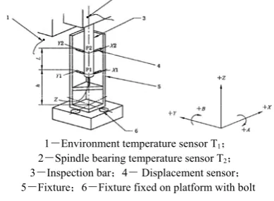
1-Environment temperature sensor T1; 2-Spindle bearing temperature sensor T2; 3-Inspection bar;4- Displacement sensor; 5-Fixture;6-Fixture fixed on platform with bolt
Figure 1. Installation diagram.
Figure 2. Measurement result of spindle thermal error in Z direction
(
) (
)
2 Y K T K
m
e = − k Y− k (16) Defining T, T0 and Rn as follows:
2 2
2 2
2 2
1 1 1 1 1 1
1 2 1 2
1 1
T
n n n n
⎡ ⎤
⎢ ⎥
⎢ ⎥
=⎢ ⎥
⎢ ⎥
⎣ ⎦
# # # # # #
(17)
2 2
0
2 2
1 1 1 1 1 1
1 2 2 1 2 2
1 3 3 1 3 3
T
⎡ ⎤
⎢ ⎥
=⎢ ⎥
⎢ ⎥
⎣ ⎦
(18)
[1 1
1]
T nR
=
"
(19)The normalized constraints of combined weights can be represented as follows:
k n
T =R (20)
By the linear algebra theory, we know that (20) is consistent linear system with three linearly independent equations. And the rest of the equations can be represented linearly by the three equations.
Let us assume thatR3=
[
1 1 1]
, and one of its largest independent linear equations can be represented as follows:0 3
T k=R (21) According to the calculation method of the literature [10], the constrained least squares estimate of k is written as follows:
* 1
(
1 1 *0 0 0 0 3
( T ) T[ T ) T
k k= − K K T T K K T− − ⎤ ⎡− T k −R⎤
⎦ ⎣ ⎦ (22) Here, K is column full rank matrix.
B. Predicting Variable Weights with GM(1,1) Model After calculating combined weights of each single predicting model at time t(t=N), we should determine combined weights at time t+1 so as to obtain combined prediction values. Since non-negativity and isometry of the weight vector, we use GM(1,1) model to predict the combined weights.
Assuming the weight vector of AR(p) model before time t is α0={α0(1),α0(2),…α0(t)}, the accumulative
sequence will be α1{α1(1),α1(2),…α1(t)}.
Here,
( )
( )
1
1 k 1
j
k j
α α
=
=
∑
(23) Accumulative sequence α1 satisfies the following greydifferential equation:
( )
( )
( )
( )
1
1
1 0
d d
1 1
t
a t b
t
α α
α α
⎧
+ =
⎪ ⎨
⎪ =
⎩
(24)
Here, a and b are parameters to be estimated. Using the least squares estimate, we can obtain discrete time response function of GM(1,1) model.
(
)
( )
1 k 1 0 1 b eak b
a a
α + =⎛α − ⎞ − +
⎜ ⎟
⎝ ⎠ (25) After inverse accumulated generating operation (IAGO) of sequence α1
(
k+1)
, we can predict the values ofweight vector.
(
)
(
)
( )
( )
0 k 1 1 k 1 1 k 0 1 b 1 e ea ak
a
α + =α + −α =⎛α − ⎞ ⎡ − ⎤ −
⎜ ⎟ ⎣ ⎦
⎝ ⎠ (26)
According to the model we get the weight vector α(t +1) at time t+1, and the weight vector of LS-SVM model is as (27).
( )
t 1 1( )
t 1β + = −α + (27)
IV. SPINDLE THERMAL ERROR MODELING OF FIVE-AXIS
MACHINING CENTRE
Taking a five-axis vertical machining centre as experimental subject, the thermal error of spindle is measured. Measuring instrument installation is shown in figure 1.
T1 and T2 are temperature sensors. T1 is used to
measure environment temperature, while T2 is installed near the location of the spindle bearing to measure its temperature rise. X1, X2, Y1, Y2 and Z are displacement sensors planted along three perpendicular axis parallel to the machine direction to measure thermal drift errors along the X, Y, Z direction. Sensor placement point P1 is
220mm apart from the platform, and the distance between P1 and P2 is 150mm.
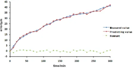
Figure 3. Modeling result of spindle thermal error in Z direction
A. LS-SVM Modeling of Thermal Error
On the basis of the collected thermal error, we can calculate the parameters a and b of LS-SVM model. Using dynamic adaptive algorithm, model parameters are obtained in (28).
γ=56.2,σ2 =71.4 (28)
According to (5), we get the values of parameters a and b of LS-SVM model.
(
132.52, 476.73, 563.28,146.54, ,187.73)
14.52
a b
= − −
=
" (29)
B. AR(p) Modeling of Thermal Error
Since the change trend between thermal error of machine tools and temperature is obvious, the nonstationary sequence should be smoothed. After that, time series analysis model is used to fit it. Fitting formula is shown in (30).
AR( )
( )
0
p s t
x t =C +C T x+ (30)
Here, C0 is constant; Cs is the temperature coefficient; T
is temperature; xt is remnant.
Taking the 30 samples of thermal error experimental data in (25), we can work out the least squares estimate of C0 and Cs based on the linear regression equation.
l0 194.83,ls 1.762, 67.21 ss
C = C = − R = (31)
Here, Rss is residual sum of squares.
Upon inspection, the residual sequence is not white noise, so we fit it with time series analysis model after zero mean smooth processing and stationary test. By the minimum and final prediction error criterion of model order, remnants {xt} obey to AR(1) model.
1 1
'
'
t t t
x
=
ϕ
x
−+
a
(32) Based on the sample estimates of auto-covariance function and autocorrelation function, we can obtain the moment estimation1
ϕ and 2
a
σ of autoregressive parameter ϕ1 and variance of αtin the AR(1) model by
solving Yule-Walker equation.
2
1 0.213, a 1.379,Rss 61.56
ϕ = σ = = (33)
So the time series analysis model of thermal error is as follows:
AR( )
( )
AR( )( )
1
153.33 0.213 1 1.762 0.375
p p t t
x t = + x t− − T + T−
(34) C. Determination of Variable Weights
Using the method of determining variable weight coefficients in chapter III.B, we obtain the weight vector ofα and β.
α={0.67,0.72,0.65,…,0.58} (35) β={0.33,0.28,0.35,…,0.42} (36) Therefore the weights α(t+1) and β(t+1) at time t+1 can be worked out by predicting variable weights using GM( 1,1).
V. RESULT AND ANALYSIS OF VARIABLE-WEIGHT
COMBINATION PREDICTION
The variable-weight combination prediction model is applied to a five axis vertical machining centre. It’s used in the prediction of spindle thermal error of Z direction, which is shown in figure 3.
From figure 3, we know that the model has high accuracy. So it can predict the variation trend of thermal error effectively.
To analyze the prediction accuracy of variable-weight combination prediction model and single prediction model with LS-SVM and time series analysis model, we work out average residual value e and residual variance δ of them respectively. Comparative analysis result is shown in table 1.
From table 1 we know that variable-weight combined prediction model can get higher prediction accuracy than single modeling method with LS-SVM and time series analysis.
VI. CONCLUSION
Since the cause and change law of thermal deformation error in machining process are very complex, single prediction model will result in lower prediction accuracy. The work proposed the variable-weight combined prediction model by integrating LS-SVM and time series analysis. GM (1, 1) model was used to predict the variable weights. Application of the grey variable-weight combined model on a five axis vertical machining centre indicated that it can get higher prediction accuracy than single modeling method. So it can be applied in online compensation of the thermal errors CNC machine tools effectively.
TABLE I
ACCURACY COMPARISON OF DIFFERENT MODELS
Parameter
Modeling method
LS-SVM AR(p) combination predictionvariable-weight
e/µm 1.15 -0.43 -0.04
ACKNOWLEDGMENT
This work was supported in part by the national science and technology major projects of China (2013ZX04005-012).
REFERENCES
[1] Ramesh, R., Mannan MA, Poo AN.Error Compensation in Machine Tools--a Review Part II--Thermal Errors.
International Journal of Machine Tools and Manufacture, Vol. 40, 2000, No 9, 1257-1284.
[2] Ni J. A Perspective Review of CNC Machine Accuracy Enhancement through Real-time Error Compensation. China Mechanical Engineering, Vol. 8, 1997, No 1, pp. 29-33.
[3] Liu Y.W., Q. Zhang, X.S. Zhao. Muti-body System-based Technique for Compensating Thermal Errors in Machining Centers. Journal of Mechanical Engineering, Vol. 38, 2002, No 1, pp. 127-130.
[4] Yan J.Y., J.G. Yang. Application of Grey(X,N) on CNC Machine Thermal Error Modeling. China Mechanical Engineering, Vol. 20, 2009, No 11, pp. 1297-1300. [5] Zhang Y. J.G. Yang. Modeling for Machine Tool Thermal
Error Based on Grey Model Preprocessing Neural Network. Journal of Mechanical Engineering, Vol. 47, 2012, No 7, pp. 134-139.
[6] Lin W.Q., J.Z. Fu, Z.C. Chen. Modeling of NC Machine Tool Thermal Error Based on Adaptive Best-fitting
WLS-SVM. Journal of Mechanical Engineering, Vol. 45, 2009, No 3, pp. 178-182.
[7] Song Q., A.M. Wang, Y.S. Zhang. The combination Prediction of BTP n Sintering Process based on Bayesian Framework and LS-SVM. TELKOMNIKA Indonesian Journal of Electrical Engineering, Vol. 11, 2013, No 8, pp. 4616-4626.
[8] Song Q., A.M. Wang, Y.S. Zhang. The combination Prediction of BTP n Sintering Process based on Bayesian Framework and LS-SVM. TELKOMNIKA Indonesian Journal of Electrical Engineering, Vol. 11, 2013, No 8, pp. 4616-4626.
[9] Yang Z.M., C.B. Zhang. Application of Time Series Analysis in Fault Diagnosis of Auto Gearbox.Transactions of the Chinese Society for Agricultural Machinery, Vol. 31, 2000, No 3, pp. 92-95.
[10]Tang X.W, Y. Zeng. Variable Weight Combination Forecasting Model. Forecaste, 1993, No 3, pp. 46-48.
Zhiming Feng received the master’s degree in Mechanical
Designing and Manufacturing Automation from Xihua University. He currently studies for a Ph.D. degree in Mechanical Engineering at Sichuan University. His recent interests focus on computer integrated manufacturing system.
Guofu Yin received the Ph.D. degree in Mechanical