Analysis of filtering solutions based on the
‘FastSLAM’ framework
Wu Zhou
Research Centre of Electromechanical Technology, Zhejiang Normal University, Jinhua, Zhejiang, China [email protected]
Chunxia Zhao
College of Computer Science and Technology, Nanjing University of Science and Technology, Nanjing, China [email protected]
Abstract—The joint state is factored into a path component
and a map component in the FastSLAM framework, which reduces the computational complexity greatly. Among all the filtering solutions based on the FastSLAM framework, the particle filtering solution and the kalman filtering solution are the two most important series. Analysis of the two filtering SLAM solutions is made in this paper. And the conclusions are as follows: Firstly, the kalman filtering SLAM solution is superior to the particle filtering SLAM solution in computational complexity. Secondly, the two filtering SLAM solutions perform similarly well in estimation accuracy. In addition, the kalman filtering SLAM solution and the particle filtering SLAM solution are evaluated with the ‘Victoria Park Dataset’, which is a bench mark dataset in the SLAM community. The experimental results show that the association between observations and estimated features is vital to the accuracy and convergence of the FastSLAM framework based solutions. Thus, special concern should be paid to reliability and stability of the data association process in SLAM.
Index Terms—Simultaneous Localization and Map
Building (SLAM); FastSLAM; Particle Filter; Kalman Filter; Analysis
I. INTRODUCTION
The Simultaneous Localization and Map Building (SLAM) problem means that a robot is placed at an unknown location in an unknown environment and the robot incrementally builds a consistent map of this environment while simultaneously determining its location within this map. Smith, Cheeseman [1] and Durrant-Whyte [2] established a statistical basis for describing landmarks in a map and manipulating geometric uncertainty. Smith, Self and Cheeseman [3] firstly presented the SLAM solution. In Ref. [3], EKF (extended kalman filter) was used to estimate the pose of the robot and the location of landmarks simultaneously.
As to the SLAM of a nonlinear system, EKF-SLAM [3, 4] and FastSLAM [5, 6] are the two general solutions. In the FastSLAM framework, the joint SLAM state is partitioned into a path component and a conditional map component aiming at shrinking the dimension of the state vector. The robot pose is represented by weighted
samples, and the map is represented as a set of independent Gaussians. A recursive estimate of the pose state is realized with a sequential particle filter and the map state with EKF. C. Kim and others [7] made use of UT (Unscented Transform) to improve the performance of the FastSLAM 2.0 algorithm. However, they did not discuss the critical issue — computational complexity. Mean extended kalman filter (MEKF) [8] and unscented kalman filter (UKF) [9] are two nonlinear kalman filters. Fast Kalman SLAM [10] inherits the ‘factorization’ idea of FastSLAM. And the robot pose is estimated with MEKF [8] or UKF [9], instead of a particle filter, while the feature’s location is estimated with EKF.
The FastSLAM framework is a widely used framework in SLAM. Particle filters and kalman filters are the two main filter families in FastSLAM solutions. Analysis of the particle filtering solution and the kalman filtering solution based on the FastSLAM framework are made herein.
II. THE PROBABILISTIC FORM OF SLAM
At time instant k, the robot pose and map could be
described as xk and m respectively. The SLAM problem means the computation of the probability distribution p(xk,m|z1:k,u1:k). The posterior probability
distribution could be formulated as (1).
1 1 at time Posterior
1 : 1 1 : 1 1 model Motion
1 model
Obervation
at time Posterior
: 1 :
1, ) ( | , ) ( | , ) ( , | , )
| ,
( ∝
∫
− − − − k−k k k k k k k k k k
k k
k p p p d
p xm z u zxm xx u xmzux
(1)
Where zk is the observation vector at time instant k.
k
u is the controlling vector, applied at time k-1 to drive
the robot to state xk . z1:k=
[
z1,",zk]
, and[
k]
k u u
u1: = 1,", .
The FastSLAM algorithm [5, 6] firstly factores the SLAM problem into a path component and a map component. Then, the map estimate is divided into M
independent feature estimates. This can be described as (2). ) , , | ( ) , | ( ) , | ( ) , , | ( ) , | , ( : 1 : 1 : 1 1 : 1 : 1 : 1 : 1 : 1 : 1 : 1 : 1 : 1 : 1 : 1 : 1 k k k i M i k k k k k k k k k k k k p p p p p u z x m u z x u z x u z x m u z m x = ∏ =
= (2)
Where, M represents the quantity of features
(landmarks).
In the particle filtering FastSLAM solution, the robot path is estimated with a particle filter. And the map of each particle is updated with a kalman filter.
A. Path estimation of FastSLAM
At time k, the posterior probabilistic distribution
) , | ( 1:k 1:k 1:k
p x z u of the robotic path is approximated with a set of particles
{
}
Ni i k i
k w 1 :
1 , =
x , where i
k
: 1
x is the state of
ith particle, and
w
ki is the weight of the ith particle. Generally speaking, it is impossible to sample directly from the distribution of posterior pose. Therefore, it is necessary to sample from a proposal distribution) , | ( 1:k 1:k 1:k
q x z u , which is similar to p(x1:k|z1:k,u1:k), and to weight the samples according to the following importance weight in (3).
) , | ( ) , | ( : 1 : 1 : 1 : 1 : 1 : 1 k k i k k k i k i k q p w u z x u z x
= (3)
It is reasonable to assume that the proposal takes the following form: ) , | ( ) , , | ( ) , |
( 1: 1: 1: = −1 1:−1 1:k−1 1:k−1 i k k k i k i k k k i
k q q
qx z u x x z u x z u
The weight of ith particle can be updated with the
following recursive equation:
i k k k i k i k k k i k k k i k i k w q p p w 1 1 1 : 1 1 : 1 1 : 1 : 1 : 1 : 1 ) , , | ( ) , | ( ) , | ( − − − − − = u z x x u z x u z x (4)
In FastSLAM 2.0, p(xk|xk−1) is merged with the observation at time k to obtain the proposal distribution
) , , |
( k k1 k k
q x x − z u . Assuming the changing process of the robot pose is a Markov process, the weight of the ith
particle could be formulated as in (5).
) , , | ( ) , | ( ) | ( ~ 1 1 1 k k i k i k k i k i k i k k i k i k q p p w w u z x x u x x x z − − −
= (5)
We can obtain the normalized weight of the ith particle
with (6).
∑
= j j k i k ik w w
w ~ / ~ (6)
The pose i k
x can be obtained by sampling from the proposal distribution q(xk|xk−1,zk,uk). And its weight
i k
w can be calculated with (5). If
{
}
N i i k ik1 w 1 1 :
1−, − =
x
represents the posterior path distribution
) , |
( 1:−1 1:k−1 1:k−1
i k
p x z u at time k-1, the posterior path
distribution ( 1: | 1:k, 1:k) i
k
p x z u at time k can be
represented as the sample set
{
}
N i i k ik w 1 :
1 , =
x , which is made up of
{ }
Ni i
k 1 1 :
1 − =
x , i
k
x , and i k w .
B. Map estimation of FastSLAM
Every particle has its own map in particle filtering solution based on the FastSLAM framework. Assuming features in the map are mutually independent, the map could be represented as a set of independent Gaussians.
) , , ˆ | ( ) , , ˆ |
( 1: 1: 1: 1 : 1 : 1 :
1 i k k k
M
i k k
k p
p m x z u m x z u
= ∏
= (7)
Where mi represents the ith landmark. M is the quantity of landmarks in a map. The mapping problem is an estimation of the mean and covariance of every landmark mi in the map. Thus, the map can be described as (8).
{
μ P μM PM}
m = 1, 1," , , (8)
Where μi
and Pi
are the mean and covariance of
i
m respectively. Then, EKF could be used to update the estimation of the features in the map. The mean and covariance of observed landmarks is computed recursively with (9) and (10), while the mean and covariance of non-observed landmarks remains in the same state at the previous time instant.
)] ( [ 1 1 i k i k i k i k i
k = μ − + K z −h μ −
μ (9)
T l l l
1 ( )
i i i i k i
k P K S K
P = − − (10)
Where i k
z is the actual observation of ith landmark at
time k, while ( 1)
i k
h μ − is the predicted observation. i
l
S and i
l
K are computed with the following equations.
k i
k i
h
hP R
Sl =∇ l −1∇ lT+ (11)
1 l T l 1
l = −∇ ( )−
i i k i h S P
K (12)
Where ∇hl is the Jacobian matrix of hl evaluated at
i k−1
μ .
IV. KALMAN FILTERING SOLUTION BASED ON THE FASTSLAM FRAMEWORK
filter in Ref. [6] turns into a kalman filter when there is only one particle. EKF is used to estimate the pose state in FastSLAM 2.0 with M=1 particle. ‘Fast EKF SLAM’
is introduced herein to represent the FastSLAM 2.0 [6] with M=1 particle. We hold that ‘Fast EKF SLAM’
should be regarded as a special kalman filtering SLAM solution, instead of a particle filtering SLAM solution.
When EKF is used for pose estimation in nonlinear SLAM, a severe error may occur with the linearization process. As for MEKF, the kalman gain is amended to reduce the linearization error. UKF achieves nonlinear filtering through statistical approximation. Particle filter (PF) maintains a large number of particles. The linearization error is lessened by adjusting the particles’ weight. Fast Kalman SLAM [10] inherits the ‘factorization’ idea of FastSLAM. With a view of the computational complexity of the particle filter, MEKF [8] or UKF [9], instead of a particle filter, is used to estimate the robot pose recursively.
A. The path estimation of Fast Kalman SLAM solutions
The path estimate is composed of pose estimates from prior time instances. EKF [3], MEKF [8] or UKF [9] is used to estimate the robot pose. MEKF is used to estimate the robot pose in Fast Kalman SLAM 1.0 [10], while UKF is used in Fast Kalman SLAM 2.0 [10]. MEKF and UKF are two kalman filters for the nonlinear SLAM problem. In MEKF, observation is used to revise the kalman gain. In UKF, UT is used to approximately compute the kalman gain. If the observation is reliable, MEKF is an effective filter for SLAM. UKF is applicable to severely nonlinear robotic systems.
Estimating the robot pose with EKF
The robot pose is assumed to be a Gaussian. At time k,
the robot pose is described as N(xˆk,Pk). The mean xˆ k and covariance Pk are estimated with EKF. The estimating process is divided into a time-updating step and an observation-updating step.
The initial mean and covariance are given in advance. For example, we assume xˆ0 = x0 and P0 =P0. x0
and P0 are determined by experimental conditions. Time-update
The predicted value of pose state at time k-1 is
formulated as the following equation.
1 ,
ˆ
kk−x
=f
(
x
ˆ
k−1,
u
k)
The covariance of prediction at time k-1 could be
described in the following equation.
k k
k
k fP f Q
P − =∇ −∇ T+
1 1 ,
Where ∇f is the Jacobian matrix of f evaluated at
1 ,
ˆkk−
x . Qk is the covariance of prediction noise.
The predicted value of observation at time k-1 is
formulated as follows:
) ˆ ( ˆk,k−1=h xk,k−1
z
Observation-update
The estimated pose is formulated as (13).
)) ˆ ( ( ˆ
ˆk = xk,k−1+K zk −h xk,k−1
x (13)
The estimated variance is computed with (14).
T 1
, KS K
P
Pk = kk− − k (14)
Where
k k
k
k hP h R
S =∇ ,−1∇ T+ (15)
1 T 1
, −∇ −
=Pkk h Sk
K (16)
In above equations, ∇h is the Jacobian matrix of h
evaluated at
i k
k, 1
ˆ
−x
. Rk is the covariance of the
observation noise.
Estimating the robot pose with MEKF
Mean extended Kalman filter (MEKF) [8] reduces linearization error by revising the kalman gain. Its basic idea is shown as Fig. 1.
Figure 1. Graphic fundamental of MEKF
For EKF, the kalman gain was calculated with the Jacobian matrix of h(x) at xˆk,k−1, which is x(0) in Fig.
1. For MEKF, the mean of ∇hx=xˆk,k−1 and ∇hx=xk is
used to compute the kalman gain. It can be seen from Fig. 1 that the dotted line, instead of the solid line, at x(0) is used for linearization. And the slope of the dotted line is the mean of the slope of the solid line through x(0) and the slope of the solid line through xk.
2 / ) ( x xˆk,k1 x xk
k = ∇h = − +∇h =
H (17)
In (17), the physical meanings of ∇hx=ˆxk,k−1 and
k x x h =
∇ are the slopes of h(x) at xˆk,k−1 and xk respectively.
The observation of relative location between the robot and a feature, and the observation of the robot bearing are needed to compute ∇hx=xk . When the robot is moving,
is only used in the case that the robot is rather stable or static.
If MEKF is used to estimate the robot pose, the estimated pose and variance are computed with (13) and (14) respectively. However, the kalman gain K in (13) and (14) is formulated as (18).
1 T 1
,− −
=Pkk HkSk
K (18) Where Hk is computed with (17) and Sk are computed
with (19). k k k k k
k H P H R
S = ,−1 T+ (19)
Estimating the robot pose with UKF
In UT (Unscented Transform) [9], a set of weighted sigma points are used to represent the stochastic characteristics of the state vector. The new stochastic characteristics, such as mean and covariance, are reconstructed with these sigma points. UKF [9] is constructed by bringing the mean and covariance obtained with UT into the recursive process of a kalman filter. The essence of UKF [9] is that 2n+1 sigma points
are used in the recursive computation. ‘Approximate probability’ is used to achieve non-linear filtering.
When UKF is used to estimate the robot pose, the predicted pose and variance in the prediction are obtained with UT. The estimated pose and variance are computed with (13) and (21) respectively in the observation-updating step. The Kalman gain K is computed with (20).
1
)
( + −
=Pxz Pzz Rk
K (20)
T 1
, K(P R )K
P
Pk = kk− − zz + k (21)
Where T 1 , 1 , 1 , 1 , 2 0 ) c ( [( ) ˆ ][( ) ˆ ] − − − − = − −
=
∑
kk i kk kk i kk ni i z
z w Z z Z z
P (22)
T 1 , 1 , 1 , 1 , 2 0 ) c ( [( ) ˆ ][( ) ˆ ] − − − − = − −
=
∑
kk i kk kk i kk ni i z
x w X x Z z
P (23)
B. Map estimation of Fast Kalman SLAM solutions
In the SLAM problem, the path estimate and map estimate are interrelated. Every feature in the map meets a two-dimensional Gaussian distribution in the FastSLAM framework. EKF outweighs MEKF and UKF in computational complexity. Therefore, the estimate of the observed features in map is generally updated with EKF in Fast Kalman SLAM solutions.
V. EXPERIMENTS
A. Experimental models
The intelligent vehicle, shown in Fig. 2, of the ACFR (Australian Centre for Field Robotics) [11] is used as the experimental model. Experimental data is collected with a laser range finder, a GPS, and an inertial sensor. The laser range finder was used to observe landmarks. The inertial sensor is used to collect the vehicle’s speed and
steering direction. And the GPS data was collected to provide ground truth. The inertial sensor collected a measurement every 25 ms (40 Hz). And the laser measurements were collected every 214 ms.
Figure 2. The intelligent vehicle for data collection
Motion Model
The motion model is shown as Fig. 3. The vehicle’s pose is described as (24).
T v v v
v(k)=[x (k) y (k) φ (k)]
X (24)
Where xv(k) , yv(k) , and
φ
v(k) respectivelyrepresent the x-coordinate, y-coordinate and bearing of
the intelligent vehicle at time k.
Figure 3. Motion model of the intelligent vehicle
The motion model is formulated as (25).
X k k k k k k k k k k k k L v T b a L v v T y b a L v v T x y x η + ⎥ ⎥ ⎥ ⎥ ⎥ ⎥ ⎦ ⎤ ⎢ ⎢ ⎢ ⎢ ⎢ ⎢ ⎣ ⎡ Δ + − + Δ + + − Δ + = ⎥ ⎥ ⎥ ⎦ ⎤ ⎢ ⎢ ⎢ ⎣ ⎡ + + + ) tan( ))) sin( ) cos( )( tan( ) sin( ( ))) cos( ) sin( )( tan( ) cos( ( c c c c c 1 1 1 α φ φ φ α φ φ φ α φ φ (25) ) tan( 1 e c α L H v v −
= (26)
Where vc is velocity of the intelligent vehicle’s back
back left wheel. α represents the steering angle of the intelligent vehicle. ηX represents the noise of motion.
Observation Model
The observation model is formulated as (27).
Z v
k v k i k
v k i k
v k i k v
k i k
k k k
x x
y y
y y x
x r
η
z +
⎥ ⎥ ⎥
⎦ ⎤
⎢ ⎢ ⎢
⎣ ⎡
+ − − −
− + −
=
⎥ ⎦ ⎤ ⎢ ⎣ ⎡
=
2 π )
arctan(
) (
) (
, , ,
, ,
2 , , 2 , ,
φ θ
(27)
Where (xk,i,yk,i) and (xk,v,yk,v) are coordinates of the ith landmark and the intelligent vehicle at time k.
k
r
represents the distance between the vehicle and thelandmark, and
θ
k represents the landmark’s bearing.k
r
andθ
k are obtained with a laser range finder. ηzrepresents the observation noise.
B. Simulative experiments
Simulative experiments are carried out in MATLAB to compare the performance of Fast Kalman SLAM and that of FastSLAM 2.0. Parameters of the simulative environment are as follows. Dimension of the simulative environment is 60 m × 55 m. Speed of the robot is 3 m/s, and the maximum rudder angle is 90°. The speed error is 0.3 m/s, and the rudder angle error is 3°. The scanning range and frequency of the laser range finder are 30 m and 5 Hz respectively. The range error and bearing error of laser range finder are 0.1 m and 1° respectively.
Fig. 4 shows the simulation results of Fast Kalman SLAM 1.0 and FastSLAM 2.0. In Fig. 4, the true path is the solid line starting at (0, 0). The dotted line is the estimated path of Fast Kalman SLAM 1.0, while the dashed line is the estimated path of FastSLAM 2.0. And the circle represents the true location of a feature in the simulative environment. ‘+’ and ‘•’ respectively represent the estimated location of a feature for FastSLAM 2.0 and Fast Kalman SLAM 1.0.
Figure 4. Path estimate and map estimate in the simulative environment
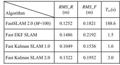
As can be seen from Fig. 4, FastSLAM 2.0 and Fast Kalman SLAM 1.0 perform nearly in estimation accuracy. In order to assess the performance of the two algorithms more accurately, 20 Monte Carlo trials are carried out, and the results are recorded in Table 1. The root mean square error (RMSE) of the estimated location of the robot and the one of the estimated location of features are RMS_R and RMS_F in Table 1. Tav in Table 1
represents the average running time of an algorithm. The quantity of particles is one hundred in the simulative experiments. A resampling strategy is introduced when the number of effective particles falls below fifty. The running time of FastSLAM 2.0 is proportional with the quantity of samples. This causes the computational complexity of FastSLAM 2.0 to be stringent. And the average running time of FastSLAM 2.0 is almost one hundred times of the one of Fast Kalman SLAM 1.0. Fast EKF SLAM is sorted herein into a kalman filtering solution based on the FastSLAM framework, while Fast EKF SLAM is treated in Ref. [6] as a special case of FastSLAM 2.0 with M=1 particle. FastSLAM 2.0 also
falls behind Fast EKF SLAM and Fast Kalman SLAM 2.0 in computational efficiency. Fast Kalman SLAM 1.0 is computationally superior to Fast Kalman SLAM 2.0 for the reason that MEKF is more computationally efficient than UKF. Fast EKF SLAM is the most efficient solution of all. In addition, the robot motion in the simulative environment lasts for 34.6 seconds. This means that kalman filtering solutions based on the FastSLAM framework are suitable for real-time SLAM applications.
As can be seen from Table 1, estimation accuracy of FastSLAM 2.0 and that of kalman filtering solutions are near. And Fast Kalman SLAM 1.0 performs best in estimation accuracy for its lowest RMS_R and RMS_F.
Table 1. Comparison of the performances of Fast Kalman SLAM solutions and FastSLAM 2.0
Algorithm
RMS_R
(m) RMS_F(m) Tav(s)
FastSLAM 2.0 (M=100) 0.1252 0.1821 188.6
Fast EKF SLAM 0.1486 0.2192 1.5
Fast Kalman SLAM 1.0 0.1049 0.1536 1.6
Fast Kalman SLAM 2.0 0.1322 0.1952 3.0
C. Experiments with ‘Victoria Park Dataset’
‘Victoria Park Dataset’ [11] is used to evaluate the performance of Fast Kalman SLAM solutions and FastSLAM 2.0. Fig. 5(b) indicates the SLAM results of FastSLAM 2.0. And Fig. 5(c) indicates the SLAM results of Fast Kalman SLAM 1.0.
pedestrians are treated as false features.
In Fig. 5(a), the solid line is the path estimated with the odometer measurements. It can be seen in Fig. 5(a) that the estimated path diverges significantly. Fig. 5(b) shows the SLAM results of FastSLAM 2.0 [6] with one hundred particles. Fig. 5(c) shows the SLAM results of Fast Kalman SLAM 1.0. In Fig. 5(c), the estimated path is nearly consistent with the GPS records. And the estimation accuracy of Fast Kalman SLAM 1.0 in Fig. 5(c) is close to that of FastSLAM 2.0 in Fig. 5(b). It can be concluded from Fig. 5 that Fast Kalman SLAM 1.0 qualifies for the estimation accuracy. The observation bearing is needed for Fast Kalman SLAM 1.0. In testing, the observation bearing is often of severe error. Thus, the bearing sensor should be stable or static when the bearing information is measured. There is no observation bearing in the ‘Victoria Park Dataset’. Thus, the estimated bearing information, instead of observation bearing, is used in the experiments. The SLAM results of Fast Kalman SLAM 2.0 and Fast EKF SLAM with ‘Victoria Park Dataset’ are similar to those of Fast Kalman SLAM 1.0 in Fig. 5(c).
(a)
(b)
(c)
Figure 5. Experimental results of Fast Kalman SLAM 1.0 and FastSLAM 2.0 with the ‘Victoria Park Dataset’
The running time of Fast Kalman SLAM 1.0 and FastSLAM 2.0 evaluated with ‘Victoria Park Dataset’ are recorded in Table 2. One hundred particles are used in FastSLAM 2.0. It can be seen from Table 2 that the running time of FastSLAM 2.0 is longer than that of Fast Kalman SLAM 1.0. This indicates that Fast Kalman SLAM 1.0 performs better in computational efficiency. The moving process of the intelligent vehicle for data acquisition lasts about one thousand and five hundred seconds. And the moving time of the intelligent vehicle is much longer than the running time (37.8 seconds) of the Fast Kalman SLAM 1.0 algorithm. This indicates that Fast Kalman SLAM solutions are good at meeting real-time computational requirements in testing. The computer specifications in the SLAM experiments are as follows: Intel Pentium (R) Dual CPU E2200 2.2 GHz Processor, 1G RAM.
Table 2. Running time of Fast Kalman SLAM 1.0 and FastSLAM 2.0 evaluated with ‘Victoria Park Dataset’
Algorithm Time(s)
FastSLAM 2.0(n=100) 3475.1
Fast Kalman SLAM 1.0 37.8
Figure 6. SLAM results of Fast Kalman SLAM 1.0 using DJNN for data association
It can be seen from Fig. 6, in comparison with Fig. 5(c), that the estimated accuracy is improved greatly.
As for FastSLAM 2.0, when DJNN is used for the data association process, the SLAM results are similar to those shown in Fig. 6. This indicates that the performance of SLAM solutions based on the FastSLAM framework is not only determined by the filtering algorithm, but also by the data association method, which is of key importance.
VI. CONCLUSIONS
The FastSLAM framework could be used to reduce the computational complexity of the SLAM problem. Analysis of the particle filtering solution and the kalman filtering solution based on the FastSLAM framework is made above. We obtained the following conclusions: Firstly, the kalman filtering SLAM solution is superior to the particle filtering SLAM solution in computational complexity. Secondly, the two filtering SLAM solutions perform similarly well in estimation accuracy. In addition, the two filtering SLAM solutions are evaluated with the ‘Victoria Park Dataset’. The experimental results show that the association between observations and estimated features is vital to the accuracy and convergence of the FastSLAM framework based solutions. Hence, in SLAM research, special concern should be paid to reliability and stability of the data association method.
It should be noted that any data association algorithm is difficult to get correct association results over the whole SLAM process. It is recommended to employ a variety of data association algorithms for association between the observations and estimated features. Then, an appropriate assessing strategy is used to assess these association results. The most reasonable association result is selected finally. We hold that improvement of the data association method should be given enough emphasis in future SLAM research.
ACKNOWLEDGMENT
The authors would like to thank Australian Centre for Field Robotics (ACFR) of the University of Sydney and
relevant members of ACFR for the ‘Victoria Park Dataset’.
REFERENCES
[1] R. Smith, P. Cheesman, “On the representation of spatial
uncertainty,” Int. J. Robotics Research, 1987, 5(4), pp. 56 – 68.
[2] H.F. Durrant-Whyte, “Uncertain geometry in robotics,”
IEEE Trans. Robotics and Automation, 1988, 4(1), pp. 23 – 31.
[3] R. Smith, M. Self, P. Cheeseman, “Autonomous Robot
Vehicles,” New York: Springerverlag, 1990, pp. 167 – 193.
[4] J. Guivant, E. M. Nebot, “Optimization of the
Simultaneous Localization and Map-Building Algorithm for Real-Time Implementation,” IEEE Trans. Robotics and Automation, 2001, 17(3), pp. 242 – 257.
[5] M. Montemerlo, S. Thrun, D. Roller, B.Wegbreit,
“FastSLAM 2.0: An improved particle filtering algorithm for simultaneous localization and mapping that provably converges,” Proc. of the Int. Conf. on Artificial Intelligence, IJCAI, Acapulco, Mexico, 2003, pp. 1151–1156.
[6] M. Montemerlo, S. Thrun, “Simultaneous localization and
mapping with unknown data association using FastSLAM,” Proc. of IEEE International Conference on Robotics and Automation, Taipei, China, 2003, pp. 1985 – 1991.
[7] C. Kim, R. Sakthivel, W. K. Chung, “Unscented
FastSLAM: A Robust Algorithm for the Simultaneous Localization and Mapping Problem,” IEEE International Conference on Robotics and Automation. Piscataway, NJ, USA:IEEE, 2007, pp. 2439 – 2445.
[8] W. Zhou, C. Zhao, J. Guo, “The Study of Improving
Kalman Filters Family for Nonlinear SLAM,” Journal of Intelligent and Robotic Systems, 2009, 56(5) , pp. 543 – 564.
[9] S.J. Julier, J.K. Uhlmann, “A New Extension of the
Kalman Filter to Nonlinear Systems,” In the Proceeding of Aerosense:The 11th International Symposium on Aerospace/Defense Sensing, Simulation and Control,
Orlando FL, USA, 1997,vol. 3068, pp. 182 – 193.
[10]W. Zhou, C. Zhao, and M. Zhang, “Fast Kalman SLAM,”
2010 International Conference on Frontiers of Manufacturing and Design Science, Chongqing, China, 2010, Applied Mechanics and Materials, vol. 44-47, pp. 3174 – 3179.
[11]http://www-personal.acfr.usyd.edu.au/nebot/experimental_
data_ute.htm
[12]W. Zhou, C. Zhao, H. Zhang, “Dynamic Nearest Neighbor
Algorithm,” ACTA ELECTRONICA SINICA, 2010, 38(2), pp. 359 – 365
Wu Zhou was born in Hunan, China, in
Chunxia Zhao was born in Beijing,