www.ijres.org Volume 6 Issue 8 Ver.II ǁ 2018 ǁ PP. 06-11
A Feedback Problem For Heating Process
Vagif M. Abdullayev
1,2*1 Azerbaijan State Oil and Industry University, Baku, Azerbaijan; 2Institute of Control Systems, ANAS, Baku, Azerbaijan
Corresponding Author: Vagif M. Abdullayev
ABSTRACT :In this work, a class of optimal control problems for a rod (plate) heating process with feedback,
when the incoming information about the state of the process is continuously received only from its individual points, at which some temperature sensors are placed, is investigated. The heating process itself takes place in a stove at the expense of controlling the temperature inside the stove. The mathematical model of the controlled process is in both cases described by a punctual loaded parabolic type equation. In the work, we derive formulae for the gradient of the functional. Algorithms of numerical solutions to the considered problems are proposed.
KEYWORDS: Optimal control, Loaded differential equations, Non-separated conditions.
--- Date of Submission:17-10-2018 Date of acceptance: 03-11-2018
---I. INTRODUCTION
Numerous publications deal with the problems of optimal feedback control (control design) of plants (processes) with lumped and distributed parameters. The findings in the area of feedback control systems concern mostly the lumped-parameter linear plants obeying the systems of differential equations with ordinary derivatives [1–3]. The published results on the distributed-parameter systems are scarce, and they concern particular classes of problem formulations [3–8].
The present paper is devoted to a class of problems of optimal feedback control of heating of rods (plates) where the information about the process state arrives continuously only from individual points where the temperature sensors are mounted. The rods are heated in the furnace by controlling the internal temperature. Consideration was also given to the case where the observation of rod (plate) heating is carried out at individual points at predefined discrete time instants. In both cases, the mathematical model of the controlled process is reduced to the pointwise loaded parabolic equation [9–11]. The control actions are calculated from the results of the continuous or discrete observation of the process at the observation points at the predefined time instants. A numerical method based on the earlier studies of the present authors is proposed [12–15].
II. PROBLEM STATEMENT
Let homogenous rods of the length l be sequentially (or simultaneously, but independently of each other) heated in a heating stove at the expense of the temperature
(t) produced by an external source and identical in all the heating stove. Then, the process of heating each rod is described by the following differential equation of parabolic type:
( ) ( , )
, ( , ) (0, ) [0, ], ), ( )
,
(xt a2u xt t u xt xt l T
ut xx
(1)with boundary conditions
ux(0,t)
u(0,t)
(t)
, t[0,T], (2) ux(l,t)
u(l,t)
(t)
, t[0,T], (3) where 2 const0c k a
is thermal conductivity coefficient;
c
h and
k h
are reduced coefficients of heat exchange between environment and the rod in the heating stove along the length and at the ends of the rod correspondingly; h is heat exchange coefficient; k is heat conductivity coefficient;c
is specific heat coefficient;
is the density of the material.The initial temperature of the rods, for the sake of simplicity, is considered constant along their lengths, but different for each rod. At that, we have some admissible set (interval) B[B,B] of possible values of the temperature:
, ] , 0 [ , )
0 ,
(x b const B x l
and the density function
B(
b
)
of initial temperatures is given, where
B
B
B(b)db 1,
(b) 0, b B.
(5)The current temperature u(xi,t),i1,2...,L is measured at L points xi[0,l] of all the rods with the help of sensors. Depending on the values of the temperature at the sources, the current temperature
(t)is assigned inside the heating stove.Let
i,i1,2,...,L be weighting coefficients characterizing the importance of taking into account thevalues of the temperature at the measured points, at that
L i
i L
i
i 1, 0 1, 1,2,...,
1
. (6)The value
] , 0 [ , ) , ( )
( ~
1
T t t x u t
u L
i i
i
is the current value of the “averaged” temperature of the rod according to the measured data. This value is used to form a feedback control for the heating stove:
, ) , ( ) ( ) ( ~ ) ( ) , ; ( ) (
1
L
i i iu x t
t K t u t K K t
t
(7)where K(t) is control parameter defining the temperature of the heating stove. The vector
(
1,
2,...,
L), in the general case, may be a function of time, but for the sake of simplicity, we consider it to be invariable and unknown.Taking into account (7) in (1)-(3), we obtain the boundary problem of the form:
, ] , 0 [ ) , 0 ( ) , ( , ) , ( ) , ( ) ( )
, ( )
, (
1
2u xt K t u x t u x t xt l T
a t x u
L
i i i xx
t
(8)(0, ) (0, ) () ( , ) , [0, ],
1
T t t x u t K t u t
u L
i i i
x
(9)(, ) (, ) ( ) ( , ) , [0, ]
1
T t t x u t K t l u t
l u
L
i i i
x
. (10)Problem (8)-(10) is called a pointwise loaded problem, as unknown values of the phase variable at different points of the space variable are present in its right-hand side.
In practical applications, there may be certain technological constraints imposed on the control parameter K(t):
K t K
K () , t[0,T], (11)
where K,K are given upper and lower admissible values of the magnification constant correspondingly. Suppose we have the following performance criterion:
2 0 2 2
] , 0 [ 0 1
2
) ( )
( ) ; , ( ) ,
( B L T RL
B
K t K db b b K I K
J
, (12)
l
dx x U b K T x u x b
K I
0
2
) ( ) , , ; , ( ) ( ) ; ,
(
, (13)where U(x) is given function;
(x)0 is given weighting function; u(x,t;K,
;b) is the solution to boundary problem (8)-(10) in the presence of control parameters K K(t),
and of initial condition] , 0 [ , ) 0 ,
(x b x l
u ; K R RL
0 1 0 2
1 0,
0, ,
are regularization parameters satisfying (6) and (11). The case when the observation over the heating process at the points xi[0,l],i1,2...,Lx of the rod is carried out not continuously, but at given discrete moments of timeT t t L j
T t
t
L t
j[0, ], 0,1,..., , 0 0, , is of practical interest. The temperature inside the heating stove
is assigned according to the results of observation, and is constant at the interval of time between any two observations, and is determined, for example, by the formula:
.
,...,
2
,
1
)
,
[
,
,
)
,
(
)
(
11
1 j j j t
L
i
j i i
j
u
x
t
const
K
const
t
t
t
j
L
K
t
x
It is possible to make use of the “memory” to measure the values of the temperature at time using the formula
() ( , ) , [ 1, ),
1 1
1
1
1 j j
L
i j
j i ij
j u x t const t t t
K
t x
(15)where
i are weighting coefficients of the importance of taking into account the value of the temperature ati
thpoint
x
i at
th measurement at(
j
1
)
th time interval, i.e. at moments of time t ,
0,1,...,j1 .
The control problem is reduced to seeking the finite-dimensional vector of parameters )
,..., ( , ) ,...,
(K1 KLt 1 Lx
K
in case of (14), and the matrix
((
ij)),i1,...,Lx, j1,2,...,Lt in case of (15). For both cases, the computation given below is not altered significantly; that is why we consider only control of type (7).III.FORMULA FOR THE GRADIENT OF THE FUNCTIONAL OR PROBLEM
For the numerical solution to parametrical optimal control problem (8)-(13), i.e. for the determination of function K(t) and of finite-dimensional vector of parameters
, we propose to use first order optimization methods [16].From (8)-(13), taking into account the independence of the initial conditions of each other, and therefore the independence of the solution to boundary problems (8)-(10) for different initial conditions
B
b
)
0
,
(
x
u
, it follows the validity of the formula:
B
B B
B K
K
db b b K I grad
db b b K I grad
K J grad
K J grad
) ( ) ; , (
) ( ) ; , ( )
, (
) , (
.
That is why, in order to apply first order optimization methods, obtain formulas for the gradient of functional (13) taking into account boundary problem(8)-(10) involving any admissible initial condition:
u(x,0)b, x[0,l],bB. (16) When solving problem (8)-(13) numerically with the application of standard first order optimization procedures, at each step of the iteration procedure, we use the gradient of the functional. With that end in view, at the current control, it is necessary to solve loaded boundary problem (8)-(10) and the following conjugate integral-and-differential equation:
,
,..,
2
,
1
],
,
0
[
),
,
(
,
)
,
(
)
(
)
,
(
)
(
)
,
(
)
,
(
1 1 0
2
L
i
T
t
x
x
x
t
x
x
x
d
t
t
K
t
x
a
t
x
i i
L
i
i i
l
xx t
(17)
with boundary and initial conditions
(
,
)
(
)
,
[
0
,
],
)
(
2
)
,
(
x
T
x
u
x
T
U
x
x
l
(18)]
,
0
[
,
)
,
0
(
)
,
0
(
t
t
x
T
x
,
x(
l
,
t
)
(
l
,
t
)
,
x
[
0
,
T
]
, (19)and non-local jump condition at intermediate points
x
i,
i
1
,
2
,...,
L
of observation,
,...,
2
,
1
),
,
(
)
,
(
x
it
x
it
i
L
L
i
t
t
l
t
K
t
x
t
x
i x i ix
(
,
)
(
,
)
(
)
(
(
,
)
(
0
,
)),
1
,
2
,...,
. (20)Theorem. The gradient of the functional in problem (8)-(10) for admissible control parameters
),
(
t
K
K
is determined by the following formulas
(
0
,
)
(
,
)
(
)
2
(
(
)
),
[
0
,
]
,
)
,
(
)
,
(
)
,
(
)
,
(
0 1
1 2
0 1
T
t
K
t
K
db
b
t
l
t
t
x
u
a
t
x
u
dx
t
x
K
J
grad
B L
i
i i
B
l L
i
i i K
),
(
2
)
(
))
,
(
)
,
0
(
(
)
,
(
)
,
(
)
(
)
,
(
0 2
0 0
2
K
t
u
x
t
x
t
dx
a
t
l
t
dt
b
db
K
J
grad
B B
T l
(22)
where
u
(
x
,
t
)
u
(
x
,
t
;
K
,
;
b
),
(
x
,
t
)
(
x
,
t
;
K
,
;
b
)
are the solutions to the direct and conjugate boundary problems (8)-(13)and(17)-(20) correspondingly at given initial admissible condition u(x,0)b.IV. NUMERICAL SCHEME OF SOLUTION TO THE PROBLEM
Formulas (17)-(20) for the gradient of the functional of problem (8)-(13) can be obtained using methods of grids [15] or method of lines over time for reducing the initial problem to an optimal control problem with respect to a system of ordinary loaded differential equations involving non-local boundary conditions [13,17]. Then, applying necessary optimality conditions obtained in the work [12] to these problems, and passing to limit when the step of discretization over time tends to zero, we can obtain formulas (17)-(20). Below, we propose to use method of lines to numerically implement the iteration method of gradient projection, namely, to solve the boundary problems: direct (8)-(11) and conjugate (17)-(20). To solve the optimal control problem for the loaded system of differential equations involving non-local boundary conditions, we use the numerical method proposed in the works [13, 14,17].
In the domain , introduce the lines tssht, s0,1,...,Nt, ht T Nt and notations .
,..., 1 , 0 ), ( ,
) , ( )
( t s t t
s x u x sh K K sh s N
u Approximate boundary problem (8)-(10) by a boundary problem with respect to the following loaded system of
N
t ordinary differential equations involving non-local boundary conditions:0
)
(
1
)
(
)
1
(
)
(
1 1
2
s i
L
i i s s
t s t
s
x
h
u
x
h
u
K
u
x
u
a
, (23),
,...,
2
,
1
,
)
(
)
(
)
(
,
)
(
)
0
(
)
0
(
1 1
t L
i
i s i s s
s
L
i
i s i s s
s
N
s
x
u
K
l
u
l
u
x
u
K
u
u
(24)
]
,
0
[
,
)
(
0
x
b
B
x
l
u
. (25)Target functional (13) is approximated, for example, by the formula
Li
oi i N
s s l
t N
t
t
x
U
x
dx
h
K
K
u
x
b
K
I
1
2 2
1
0
2 0 0
1
2
(
)
(
)
)
(
)
(
)
(
)
;
,
(
(26)The obtained optimal control problem lies in determining (Nt L) dimensional vector of parameters )
,..., , ,..., ( ) ,
(K
K1 KNt
1
L . In order to solve this problem using gradient projection method, give formulas of the gradient of functional (26):
L N
I I K
I K
I b K I grad
t
; ) ,..., , ,...,, (
1 1
.
Conjugate boundary problem (17)-(20) is also approximated with the application of method of lines by loaded second order ordinary differential equations involving non-local boundary conditions
0
)
(
)
(
)
(
1
)
(
)
1
(
)
(
0 1
1
2
l L
i
i i
s s s
t s
t
s
x
h
x
h
x
K
x
dx
x
x
a
, (27)L
i
l
K
x
x
i s i s s ss
(
)
(
)
(
(
)
(
0
)),
1
,
2
,...,
, (29)which are solved successively from
s
N
t
1
tos
1
provided that
( ) ( )
) ( 2 )
(x x u x U x
t
t N
N
,x
(
0
,
l
)
. (30)Then, the components of the gradient of the functional of problem (23)-(26) are determined by the approximation of formulas (21) and (22) in the following way:
,
,..,
2
,
1
),
(
2
)
(
)
0
(
)
(
)
(
0 1
0
2 1
t s
B
l
s s
s i
s L
i i t s
N
s
K
K
db
l
a
dx
x
x
u
h
dK
dJ
.
,...,
2
,
1
),
(
2
)
(
)
0
(
)
(
)
(
0 1
0
2 1
L
i
db
l
a
dx
x
x
u
K
h
d
dJ
B
l
s s
s i
s N
s s t i
The other specific character of these boundary problems is point wise loading of equations (23) and integral loading of equations (27), as well as the presence of non-local boundary conditions (24) and (29). In the work [17], for the solution to such problems, a numerical solution method is proposed. It is based on the shift of boundary conditions, for example, from left to tight successively from point
x
0
to pointsx
1,....,
x
L,
x
l
, and as a result we obtain (L1)n (wheren
is the order of the system) algebraic equations with respect to))
(
),
(
),...,
(
(
u
sx
1u
sx
Lu
sl
. After solving this system, the initial boundary problem is reduced to a Cauchy problem that is solved from right to left. Analogical approach is proposed in [12] for integrally loaded ordinary differential equations involving non-local boundary conditions.Note that the statement of the optimal feedback control problem and the approach to its solution given above can be extended onto other classes of optimal control problem with respect to systems with distributed parameters, described by other types of partially differential equations.
V. RESULTS OF THE NUMERICAL EXPERIMENTS
We present the results of the numerical experiments that were obtained at solving the problem of feedback control of rod heating for the following data: rod length l1; heating time T 5; the coefficient of thermal conductance a1; and the coefficient of boundary heat transfer
0,01. Taking into consideration the symmetricity of heating along the rod, the points of temperature measurement were, 4 , 0 , 2 ,
0 2
1 x
x , that is, L2. The permissible upper value of the control coefficient is K 6,5, the lower one, K 0; the desired final value of the rod temperature U(x)100 and
(x)1, x[0;1].In the calculations, the set of permissible initial temperatures was varied as follows: ]
28 ; 20 [ ], 26 ; 20 [ ],
22 ; 20 [ ,
] 21 ; 20
[ 2 3 4
1 B B B
B , the sets were sampled with the step
5 ,
0 , the density function
B(b) was taken in the calculations as uniformly distributed, that is, )( 1 )
(b B B
B
. The weight coefficients were taken equal to
i 0,5,i1,2, and no optimization was carried out with respect to them, the regularization parameters were K0 3,0,
0,005. Under these conditions, exact solution of the control problem is not known and cannot be established analytically.For approximation of the direct (8)-(10) and conjugate (17)-(20) problems by a system of loaded differential equations with ordinary derivatives, the method of lines with the step
0,02 was used. At each time layer s, s1,...,m, the loaded ordinary differential equation with nonlocal conditions obtained with the use of the method of [15] was reduced to the Cauchy problems solved by the fourth-order Runge-Kutta method with the step h0,04. The precision of solution of the problem of optimal control by the method of gradient projection as defined by the variation of the functional over two last iterations was
1 0,01, that of one-dimensional optimization,
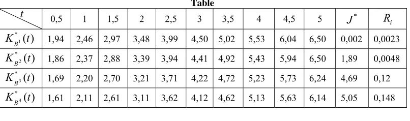
2 0,001.The table compiles the results of solving the problem of optimal control K(t) for various ranges of the set of initial rod temperatures Bi,i1,2,3,4
. Presented are the optimal values of the coefficients controlling the feedback with the step t0,5. The corresponding optimal values of the functional *
i
B
J are shown in the next to last column; and the last column shows the maximal over the rod length relative deviations of the determined rod temperatures from the desired temperature U(x)100, that is,
) ( ) ( ) , ( max
] 1 , 0
[ u xT U x U x
R
x
i
for different ranges of the initial rod temperatures Bi,i1,2,3,4. .
As can be seen from the table, with an increase in the range of possible initial temperatures of the rods, their reduction to the desired temperature by averaged control of the furnace temperature is complicated, that is, as would be expected, in this case heating controllability worsens.
Table
t
0,5 1 1,5 2 2,5 3 3,5 4 4,5 5
J
*i
R
)
(
*
1
t
K
B 1,94 2,46 2,97 3,48 3,99 4,50 5,02 5,53 6,04 6,50 0,002 0,0023)
(
*
2
t
K
B 1,86 2,37 2,88 3,39 3,94 4,41 4,92 5,43 5,94 6,50 1,89 0,0048)
(
*
3
t
K
B 1,69 2,20 2,70 3,21 3,71 4,22 4,72 5,23 5,73 6,24 4,69 0,12)
(
*
4
t
K
B 1,61 2,11 2,61 3,11 3,62 4,12 4,62 5,13 5,63 6,14 5,05 0,148VI. CONCLUSIONS
The above approach to the feedback control systems for the distributed-parameter plants can be extended to the case where the processes are described by other classes of boundary problems. Other types of observations (discrete, time interval, or their combinations) may be considered as well. This approach can be used in the control systems of the processes described by the distributed- parameter systems.
REFERENCES
[1]. Utkin V.I.( 1992) "Sliding Modes in Control and Optimization", Heidelberg: Springer. [2]. The Control Handbook, Levine, W.S., Ed., Boca Raton: CRC Press, 1996, pp. 895–908. [3]. Egorov A.I. (2004) "Introduction to the Control Theory", Moscow: Fizmatlit. [4]. Ray W.H.(1981) "Advanced Process Control", New York: McGraw-Hill.
[5]. Polyak B.T. and Shcherbakov, P.S. (2002) "Robust Stability and Control" , Moscow: Nauka. [6]. Butkovskii A.G.(1984) "Distributed-parameter Systems: Methods of Control", Moscow: Nauka.
[7]. Aida-zade K.R. (2005) "An Approach to the Design of the Lumped Control in Distributed Systems", Avtomat. Vychisl. Tekhn., No. 3, pp. 16–22.
[8]. Aida-zade K.R., Abdullaev V.M.(2012) "On an approach to designing control of the distributed-parameter processes" // Autom.
Remote Control, Vol.73, №9, pp. 1443-1455.
[9]. Nakhushev A.M. (2005) "Problems with Mixing for the Partial Derivative Equations", Moscow: Nauka. [10]. Nakhushev A.M. (1995) "Equations of Mathematical Biology", Moscow: Vysshaya Shkola.
[11]. Alikhanov A.A., Berezkov A.M., and Shkhanukov-Lafshiev, M.Kh. (2008) "Boundary Problems for Some Classes of Loaded Differential Equations and Difference Methods for Their Numerical Realization", Comput. Math. Math. Phys., Vol. 48, No. 9 pp. 1619–1628.
[12]. Abdullaev V.M., Ayda-zade K.R. (2006) "Numerical Solution of Optimal Control Problems for Loaded Lumped Systems" //
Comput. Math. Math. Phys, Vol.46, №9, pp.1487-1502.
[13]. Abdullaev V.M., Aida-zade K.R. (2004) "On the numerical solution of loaded systems of ordinary differential equations" //
Comput. Math. Math. Phys, Vol.44, № 9, pp.1585–1595.
[14]. Abdullaev V.M., Aida-zade K.R.(2014) "Numerical method of solution to loaded nonlocal boundary value problems for ordinary differential equations" // Comput. Math. Math. Phys., Vol. 54, №7, pp.1096–1109.
[15]. Abdullayev V.M., Aida-zade K.R.(2016) "Finite-difference methods for solving loaded parabolic equations" // Comput. Math. Math. Phys., Vol. 56, №1, pp.93–105.
[16]. Evtushenko Yu.G. (1982) "Methods for Solution of the Extremal Problems and Their Use in the Optimization System", Moscow: Nauka.
[17]. Abdullaev V.M. (2008) "On Using the Method of Lines for the Boundary Problem Nonlocal Conditions Relative to the Loaded Parabolic Equation", Izv. Nat. Akad. Nauk Azerb., Ser. FTMN, Vol. 28, No. 3, pp. 76–81.