Efficient Image Display for Head-Slaved Viewing of Virtual Environments

(1)

Efficient Image Display for Head-Slaved

Viewing of Virtual Environments

Amela Sadagic

A dissertation submitted in partial fulfillment of the requirements for the degree of

Doctor of Philosophy

of the

University of London.

Department of Computer Science University College London

(2)

ProQuest Number: U642073

All rights reserved

INFORMATION TO ALL USERS

The quality of this reproduction is dependent upon the quality of the copy submitted.

In the unlikely event that the author did not send a complete manuscript

and there are missing pages, these will be noted. Also, if material had to be removed,

a note will indicate the deletion.

uest.

ProQuest U642073

Published by ProQuest LLC(2015). Copyright of the Dissertation is held by the Author.

All rights reserved.

This work is protected against unauthorized copying under Title 17, United States Code.

Microform Edition © ProQuest LLC.

ProQuest LLC

789 East Eisenhower Parkway

P.O. Box 1346

(3)

‘T

ell me and I I I forget.

Show me and I may remember.

Xnvolve me and I I I understand.

’

(4)

(5)

Abstract 4 The efficient resolution of visibility in polygonal scenes was and still is one of the most demanding tasks in computer graphics. A need for faster algorithms is becoming even more important to fulfil the requirements of real-time Virtual Reality (VR) systems, and in particular immersive VR systems.

In VR systems, typically the viewpoint is changing at a greater rate than the objects within the scene. In such environments the visibility, in terms of back-to-front polygon visibility ordering, does not change dramatically from frame to frame since the viewpoint changes by small increments. In addition, stereopsis requires visibility determination for each eye; again, since the viewpoints corresponding to the eyes are so close together, coherence can be exploited to avoid the necessity of separate visibility computations for each eye. These considerations provide a sound basis from which to investigate the areas where efficiency of visibility computation might be improved. This thesis therefore considers a particular class of visibility algorithm that pre-order the scene in visibility order with respect to the viewpoint.

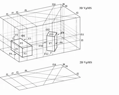
The thesis investigates the construction of visibility algorithms that makes use of the resulting view point movement coherence, where visibility information computed with respect to one viewpoint may be incrementally adjusted for a subsequent viewpoint without the necessity for a full visibility compu tation for each frame. An algorithm has been designed which supports space partitioning into cells with the property that each cell has an implicitly associated invariant visibility ordering. We introduced the concept of dynamic priority ordering. It consists of the initial ordering, generated as a linear list in the preprocessing phase, and a set of rules which define dynamic updates of the priority ordering to the one that is valid for the current viewpoint position. The entire space within which the viewpoint moves is called Viewpoint Movement Space (VpMS). This may be parameterised - it can be defined as a subset of ID (line segment or curve), 2D (convex polygon) or 3D space (convex polyhedron).

(6)

(7)

Acknowledgements 6 First of all I would like to thank my supervisor, Professor Mel Slater, for the continuous guidance and support that he has provided me during the course of my Ph.D. studies. I am very much grateful for being able to peer into the magical world of the VR, and the main responsibility of me being permanently

‘infected’ by this experience is solely his.

In Dr Yiorgos Chrysanthou I found an unlimited source of comments, discussions and above all the continuous friendship and support at difficult times of my research, and I am very much grateful for that. I have been privileged to work one Summer at the University of North Carolina at Chapel Hill supervised by Professor Frederick P. Brooks Jr, whose enthusiasm and encouragement gave an impulse in the final phase of my studies.

I am indebted to several people and institutions who provided the financial support without which I would not be able to do my PhD studies: Open Society Institute (George Soros Foundation), British Fed eration of Women Graduates, The Philip and Pauline Harris Charitable Trust and especially Lord Harris of Peckham, and my best friends Finka, Miro and Brana.

The wide network of my Bosnian, ex-Yugoslav, English and many other friends acted as my ex tended family, and my life in the UK is irreversibly marked with that experience. Adnan and Rada made my coming to London possible, and together with Mladen they are to blame for the great moments we had discovering the charm of this city. Cristina, Martin, Pip, Mike, Anthony, Bob and other people from our VR group made this place friendly, and Jeremy taught me the importance of English humour as well as the use of indefinite and definite articles. Barbara and Robin Hill, immensely caring friends from Colchester, introduced me to the rich heritage of English culture and tradition. The people from “Krila” (Wings) cul tural society of students from ex-Yugoslavia, and the altruists like Dr Celia Howksworth, Dr Lisa Jardin and Dr John Gibbs are to be specially thanked.

I would like to acknowledge the people from Queen Mary and Westfield College, Department of Computer Science, where I spent my first year, especially Senior Lecturer Sylvia Wilbur for all support that she gave me. I am also indebted to the people from University College London, Department of Com puter Science, for providing me an opportunity and environment for conducting most of my Ph.D. studies and the research that I have done. I especially thank the members of my research committee, Dr Simon Arridge and Professor Bernard Buxton, for their helpful comments and suggestions, and the technical staff for helping me whenever my Indy would refuse to cooperate.

(8)

List of Figures

1.1 Conceptual model of graphics pipeline in computer g r a p h ic s ... 21

2.1 An example of the cycle with three polygons ... 31

2.2 An example of a 2D scene and the first step of BSP subdivision... 40

2.3 Complete BSP subdivision of the scene from Figure 2 .2 ... 40

2.4 Traversal of BSP tree from Figure 2 . 3 ... 40

2.5 An example of a simple (nondegenerate) and a nonsimple (degenerate) 2D arrangement . 42 2.6 An example of a simple (nondegenerate) and a nonsimple (degenerate) 3D arrangement . 42 2.7 A zone in an arrangement of l i n e s ... 43

2.8 Level of 2-cells (faces) in a simple arrangement of lin e s... 44

3.1 A simple scene with two o b j e c t s ... 47

3.2 An example of 2D VpMS and its subdivision in four c e lls ... 50

3.3 An example of the scene from Figure 3.1, and its 2D and 3D V p M S ... 52

3.4 A simple scene with two objects and smaller 3D VpMS: first level of model pruning . . 53

3.5 An example of the leaf f a c e ... 55

3.6 An example of the face with in _ su b se t... 56

3.7 An example of the face with out-Subset ... 57

3.8 An example of the face with two s u b s e t ... 58

3.9 Dynamic visibility ordering list generated for the scene and its 3D VpMS from Figure 3.3, and reference point P I ... 60

3.10 A simple scene with two objects and smaller 3D VpMS: second level of model pruning . 62 3.11 An example of two objects and 2D V p M S ... 64

3.12 Winged Edge data structure... 64

3.13 Starting set of data in WE data structure for 2D V p M S ... 65

3.14 Inserting of one line segment as a bridge into WE data s t r u c t u r e ... 66

3.15 Crossing surfaces in 2D V p M S ... 66

3.16 An example of two objects and 3D V p M S ... 67

3.17 An example of 3D VpMS and its supportive data s tr u c tu r e ... 68

3.18 Starting set of data in MWE data structure for 3D V p M S ... 69

(13)

List o f Figures 12

3.20 Crossing surfaces in 3D V p M S ... 71

3.21 An example of 2D and 3D VpMS and dynamic visibility ordering list being updated for simple path P I - P 2 ... 73

3.22 Some extreme cases of viewpoint m o v em en ts... 74

3.23 Tracking a new position of the viewpoint ... 75

3.24 Some cases of viewpoint movements in 3D VpMS ... 76

3.25 An example of single 2D VpMS, and the same VpMS in two l a y e r s ... 78

3.26 An example of single 3D VpMS, and the same VpMS in two l a y e r s ... 80

3.27 An example of two objects and ‘thin’ 3D V p M S ... 81

4.1 Two scenes and their linear BSP t r e e s ... 89

4.2 An example of simple scene and one possible BSP t r e e ... 90

4.3 A set of cells with invariant ordering, for scene and BSP tree in Figure 4 . 2 ... 90

4.4 The scene from Figure 4.2 and another possible BSP t r e e ... 90

4.5 A set of cells with invariant ordering, for scene and BSP tree in Figure 4 . 4 ... 90

4.6 An example of three BSP t r e e s ... 92

4.7 An example of simple scene and the first three steps of Min x method ( N = 3 ) ... 95

4.8 A scene from Figure 4.7: final BSP subdivision using Min x m e th o d ... 96

4.9 A scene from Figure 4.7: BSP subdivision using Min x,y m e th o d ... 97

4.10 An example of autopartitions and separating p l a n e s ... 99

4.11 An example of a set of convex objects and its object-based BSP t r e e ...100

4.12 An example of the situations when a simple BSP tree has to be b u i l t ...101

4.13 Constructing two object-based BSP tre e s ... 101

4.14 An example of using the autopatitions and separating planes for the same s c e n e 102 4.15 Sorting method Min x applied on object-based BSP t r e e s ...103

5.1 8Houses S c e n e ... 108

5.2 8Spheres S c e n e ... 108

5.3 Office S cen e... 109

5.4 Office Scene: close u p ... 109

5.5 London 1 S c e n e ...110

5.6 London 1 Scene: close u p ...110

5.7 London2 S c e n e ...I l l 5.8 London2 Scene: close u p ... I l l 5.9 Office Scene: size of dynamic visibility ordering list, methods Min x, Min x,y,z and VpMS Moderated Fuchs’ (data in Table 5 . 4 ) ... ...117

(14)

List o f Figures 13 5.12 Office Scene: no. faces tested: 10, methods sorted by total no. of faces (data in Table 5.6) 120 5.13 Office Scene: no. faces tested: 20, methods sorted by total no. of faces (data in Table 5.6) 121

5.14 Office Scene: no. faces tested: 30, methods sorted by total no. of faces (data in Table 5.6) 121 5.15 Office Scene: no. faces tested: 40, methods sorted by total no. of faces (data in Table 5.7) 122 5.16 Office Scene: no. faces tested: 50, methods sorted by total no. of faces (data in Table 5.7) 122

5.17 Office Scene: no. faces tested: 60, methods sorted by total no. of faces (data in Table 5.7) 123 5.18 Size of MWE data structure (data in Tables 5.15, 5.16 and 5 . 1 7 ) ... 132

5.19 Size of dynamic visibility ordering list and BSP tree (data in Tables 5.15, 5.16 and 5.17) 132 5.20 Office Scene: timing results for VpMS and BSP algorithm - VpM Sl, l i n e l (data in Table

5.24 ) ...143 5.21 Office Scene: timing results for VpMS and BSP algorithm - VpM Sl, Line2 (data in Table

5.25 ) ...143 5.22 Office Scene: timing results for VpMS and BSP algorithm - VpM Sl, Line3 (data in Table

5.26 ) ...144 5.23 Office Scene: timing results for VpMS and BSP algorithm - VpM Sl, Linel, 2500 steps

(data in Table 5 . 2 7 ) ... 146 5.24 Office Scene: timing results for VpMS and BSP algorithm - VpM Sl, Linel, 5000 steps

(data in Table 5 . 2 7 ) ... 146 5.27 Office Scene: timing results for VpMS and BSP algorithm - VpM Sl, all lines, 2500 steps

(data in Table 5 . 2 9 ) ... 150 5.30 Office Scene: timing results for VpMS and BSP algorithm - VpM Sl, all lines, 10000

steps (data in Table 5 . 2 9 ) ...150 5.31 Office Scene: timing results for BSP and VpMS algorithms, three VpMSs, no.faces

tested = 5 (data in Table 5.30) ... 153 5.32 Office Scene: timing results for BSP and VpMS algorithms, three VpMSs, no.faces

tested = 10 (data in Table 5 .3 0 ) ... 153 5.33 Office Scene: timing results for BSP and VpMS algorithms, three VpMSs, no.faces

tested = 15 (data in Table 5 .3 1 ) ... 154 5.34 Office Scene: timing results for BSP and VpMS algorithms, three VpMSs, no.faces

(15)

List o f Figures 14 5.35 Time to build MWE structure as a function of no. MWE cells created (data in Table 5.33) 159 5.36 Time to build dynamic visibility ordering list as a function of no. ordering faces created:

Office Scene (data in Table 5 . 3 4 ) ...160

5.37 Time to build dynamic visibility ordering list as a function of no. ordering faces created: Londonl Scene (data in Table 5.34) ...160

5.38 Time to build dynamic visibility ordering list as a function of no. faces tested (data in Table 5.34) ...161

6.1 Hierarchical approach applied to the scene made of seven r o o m s ... 166

6.2 An example of hybrid visibility ordering list for scene with six o b je c ts ...168

6.3 Collision detection for closed polyhedra and one VpMS la y e r...171

6.4 Collision detection for closed polyhedra and more VpMS l a y e r s ... 172

6.5 Image-based rendering: two ordering faces change their visibility s t a t u s ...174

C .l Londonl Scene: size of dynamic visibility ordering list, methods Min x, Min x,y,z and VpMS Modified Fuchs’ ... 190

C.2 Londonl Scene: size of dynamic visibility ordering list, methods Fuchs’, Mean x. Mean x,y,z and Mid d i s t ... 190

C.3 Londonl Scene: no. faces tested: 6, methods sorted by total no. of ordering faces . . . . 192

C.4 Londonl Scene: no. faces tested: 10, methods sorted by total no. of ordering faces . . . 192

C.5 Londonl Scene: no. faces tested: 20, methods sorted by total no. of ordering faces . . . 193

D. 1 Office Scene: timing results for VpMS and BSP algorithm - VpMS2, Linel (data in Table D . l ) ...198

D.2 Office Scene: timing results for VpMS and BSP algorithm - VpMS2, Line2 (data in Table D . 2 ) ...198

D.3 Office Scene: timing results for VpMS and BSP algorithm - VpMS2, Line3 (data in Table D . 3 ) ...199

D.4 Office Scene: timing results for VpMS and BSP algorithm - VpMS2, Linel, 2500 steps (data in Table D.4) ... 201

D.5 Office Scene: timing results for VpMS and BSP algorithm - VpMS2, lin e l, 5000 steps (data in Table D.4) ... 201

D.8 Office Scene: timing results for VpMS and BSP algorithm - VpMS2, all lines, 2500 steps (data in Table D.5) ... 204

(16)

L ist o f Figures IS

D.IO Office Scene: timing results for VpMS and BSP algorithm - VpMS2, all lines, 7500 steps (data in Table D.6) ... 205 D .ll Office Scene: timing results for VpMS and BSP algorithm - VpMS2, all lines, 10000

steps (data in Table D . 6 ) ...205 D.12 Office Scene: timing results for VpMS and BSP algorithm - VpMS3, Linel (data in Table

D . 7 ) ... 209 D.13 Office Scene: timing results for VpMS and BSP algorithm - VpMS3, Line2 (data in Table

D . 8 ) ... 209 D.14 Office Scene: timing results for VpMS and BSP algorithm - VpMS3, Line3 (data in Table

D . 9 ) ... 210 D.15 Office Scene: timing results for VpMS and BSP algorithm - VpMS3, Linel, 2500 steps

(data in Table D .IO )... 212 D.16 Office Scene: timing results for VpMS and BSP algorithm - VpMS3, Linel, 5000 steps

(data in Table D .IO )... 212 D.17 Office Scene: timing results for VpMS and BSP algorithm - VpMS3, lin e l, 7500 steps

(data in Table D .IO )... 212 D.IS Office Scene: timing results for VpMS and BSP algorithm - VpMS3, Linel, 10000 steps

(data in Table D .IO )... 212 D.19 Office Scene: timing results for VpMS and BSP algorithm - VpMS3, all lines, 2500 steps

(data in Table D . l l ) ... 215 D.20 Office Scene: timing results for VpMS and BSP algorithm - VpMS3, all lines, 5000 steps

(data in Table D . l l ) ... 215 D.21 Office Scene: timing results for VpMS and BSP algorithm - VpMS3, all lines, 7500 steps

(data in Table D .1 2 )... 216 D.22 Office Scene: timing results for VpMS and BSP algorithm - VpMS3, all lines, 10000

steps (data in Table D .1 2 )...216 D.23 Londonl Scene: timing results for VpMS and BSP algorithm - VpM Sl, Linel (data in

Table D . 1 4 ) ...218 D.24 Londonl Scene: timing results for VpMS and BSP algorithm - VpMS2, Linel (data in

Table D . 1 5 ) ...219 D.25 Londonl Scene: timing results for VpMS and BSP algorithm - VpMS3, Linel (data in

Table D . 1 6 ) ... 220 D.26 London2 Scene: timing results for VpMS and BSP algorithm - VpM Sl, li n e l (data in

Table D . 1 8 ) ... 222 D.27 London2 Scene: timing results for VpMS and BSP algorithm - VpMS2, Linel (data in

Table D . 1 8 ) ...223 D.28 London2 Scene: timing results for VpMS and BSP algorithm - VpMS3, Linel (data in

(17)

List of Tables

2.1 Number of k-cells in simple 2D and 3D arrangements (k = 0 ,1 ,2 ,3 )... 43

5.1 Three scenes used in experiments... 107

5.2 The scheme for the experiments related to the size of the dynamic visibility ordering list 113 5.3 Set of tables and figures that sum up the results of experiments which test the size of the dynamic visibility ordering l i s t ... 114

5.4 Size of dynamic visibility ordering list for Office Scene - classified by methods and sorted by no, tested faces (p a rti)...115

5.5 Size of dynamic visibility ordering list for Office Scene - classified by methods and sorted by no, tested faces (part2)...116

5.6 Size of dynamic visibility ordering list for Office Scene - Sort2: classified by no, faces tested, sorted by total no, of ordering faces ( p a r ti) ...118

5.7 Size of dynamic visibility ordering list for Office Scene - Sort2: classified by no, faces tested, sorted by total no, of ordering faces (part2)...119

5.8 The scheme for the experiments related to the linearity of the dynamic visibility ordering l i s t ...125

5.9 Linearity of BSP tree build for Office S c e n e ... 126

5.10 Linearity of BSP tree build for Office Scene, sorted by total no, of ord,faces generated , 127 5.11 London2 Scene: alignment of the object f a c e s ...128

5.12 Size of WE data structure for scenes with s p h e r e s ... 129

5.13 Size of MWE data structure for three s c e n e s ...129

5.14 London2: complexity of MWE for the same V p M S ... 130

5.15 Memory requirements for Office Scene (3D V p M S )... 130

5.16 Memory requirements for Londonl Scene (3D V p M S ) ... 131

5.17 Memory requirements for London2 Scene (3D V p M S ) ... 131

5.18 The scheme for the experiments related to the performance of the 2D VpMS algorithm , 134 5.19 Timing results of traversal with 2D VpMS for three scenes (no, faces tested: 5, method: Fuchs’) ... 135

(18)

List o f Tables 17 5.22 Set of tables and figures that sums up Sort2 and Sort3 of the basic results of timing ex

periment ... 139 5.23 Description of Office Scene and... its three V p M S ...140 5.24 Timing results for Office Scene: comparison of BSP tree and VpMS traversal: VpM Sl,

Linel ... 140 5.25 Timing results for Office Scene: comparison of BSP tree and VpMS traversal: VpM Sl,

L i n e 2 ... 141 5.26 Timing results for Office Scene: comparison of BSP tree and VpMS traversal: VpM Sl,

L i n e 3 ... 142 5.27 Timing results for Office Scene: comparison of BSP tree and VpMS traversal - Sort2:

VpM Sl, Linel ... 145 5.28 Timing results for Office Scene: comparison of BSP tree and VpMS traversal - Sort3:

VpM Sl ( p a r t i ) ... 147 5.29 Timing results for Office Scene: comparison of BSP tree and VpMS traversal: VpM Sl

(p a rt2 )... 148 5.30 Timing results for Office Scene: comparison of three VpMSs (Linel, p a r t i ) ...151 5.31 Timing results for Office Scene: comparison of three VpMSs (Linel, p a r t 2 ) ...152 5.32 Office Scene: Timing results for basic differences between BSP and VpMS algorithm . . 157 5.33 Time needed to build MWE structures for Office and Londonl S c e n e... 158 5.34 Time needed to build dynamic visibility ordering list for Office and Londonl Scene . . . 159

C.l Size of dynamic visibility ordering list for Londonl Scene - classified by methods and sorted by no. tested f a c e s ...189 C.2 Size of dynamic visibility ordering list for Londonl Scene - classified by no. faces tested,

sorted by total no. of ordering f a c e s ...191

D .l Timing results for Office Scene: comparison of BSP tree and VpMS traversal; VpMS2, Linel ... 195 D.2 Timing results for Office Scene: comparison of BSP tree and VpMS traversal; VpMS2,

L i n e 2 ... 196 D.3 Timing results for Office Scene: comparison of BSP tree and VpMS traversal; VpMS2,

li n e l ... 200 D.5 Timing results for Office Scene: comparison of BSP tree and VpMS traversal; VpMS2 . 202 D.6 Timing results for Office Scene: comparison of BSP tree and VpMS traversal; VpMS2 . 203 D.7 Timing results for Office Scene: comparison of BSP tree and VpMS traversal; VpMS3,

(19)

List o f Tables 18 D.8 Timing results for Office Scene: comparison of BSP tree and VpMS traversal; VpMS3,

Line3 ... 208 D.IO Timing results for Office Scene: comparison of BSP tree and VpMS traversal; VpMS3,

(20)

Chapter 1

(21)

1.1. In troduction 20

1.1 Introduction

Computer graphics is a field that is primarily concerned with computer assisted image synthesis. The new quality that graphics brought in the process of communicating between humans and computers, as well as the availability of computer graphics systems, marked the widespread and somewhere indispensable use of such systems. Namely, graphics represents the most natural way of communicating between users and computers, and also among the users of the system themselves. The use of these kinds of systems is commonly accompanied with greater efficiency and productivity. On the other hand, the technological advances made such systems affordable and available to a larger community, which was another factor that influenced the great popularity of computer graphics systems.

Virtual Reality (VR) is a medium that apart from the graphics encompasses several other sensory channels such as audio, tactile, force-feedback and others. VR goes beyond the boundaries that were reached with computer graphics systems providing even more compelling experience to humans. Com puter graphics, however, being present in all VR systems, remains an extremely important element of any such a system. The high dynamics of the pictorial change as well as the realism of its content are two essential demands that any computer graphics system has to observe if it is to be a part of a highly demanding real-time system such as a VR system.

The research that we have conducted addresses the issues of the dynamics of the pictorial change in image synthesis (rendering) of walkthrough virtual environments. More precisely, we studied the ap proaches that provide an efficient solution to one part of the graphics pipeline in computer graphics, called the visibility determination task.

In the text of this thesis we will be using the term Virtual Reality in association with the type of com puter graphics systems, the underlying concepts and the technology, while the term Virtual Environment (VE) will be used to describe a specific setting in which the participant performs his/her actions. The latter term was described in more detail in [14].

1.2 Graphics Pipeline in Computer Graphics

In order to lay out a basic setting for the research that we have conducted, we first give a brief review of the graphics pipeline in computer graphics.

(22)

1.3. Visibility Determination in Computer Graphics 21

camera, a concept that helps us define the point and the direction in 3D space from which the entire (3D)

scene will be viewed. We must also specify a view ing volume w hich describes a portion of the object

space that will be visualised at any time. In addition, interactive com puter graphics requires a definition

of the dynam ics of the environm ent - the rules of interaction am ong its elem ents and the way the user can

interact w ith that environm ent.

The graphics pipeline describes a set of com putations to be undertaken on the content of an environ

ment to accom plish the task of synthesising the im age(s). Each com putation takes one set of inform ation,

perform s certain operations on it and delivers its result to the next com putation in the pipeline. Figure 1.1

shows a scheme of a typical graphics pipeline [15]. Both com putations 1 and com putations2 consist of

several com ponents. M odelling transform ations, view ing transform ations and clipping are part of com 

p u ta tio n s!, w hile operations related to the lighting and visibility determ ination (a task that defines w hich

parts o f the environm ent are visible from the camera position and will be displayed in a final image) can

be part of either com putations! or com putations2. This depends on the approach adopted in particular

system.

object space

v iew ing

space display

environm ent. projection

space . project

com putations I

clipping com p u tation s!

Figure 1.1 ; Conceptual model of graphics pipeline in com puter graphics

A com m on approach to the rendering is to perform the entire graphics pipeline each tim e a new image

has to be produced. In real-time systems this means the same task has to be perform ed several tim es per

second, a requirem ent that presents a great challenge to the system.

1.3 Visibility Determination in Computer Graphics

Visibility determ ination represents one part of the graphics pipeline, and it is a basic task of any visibility

algorithm . It identifies what is to be displayed in the image to correspond exactly to what can be seen in the

scene through the synthetic camera in every frame. A lthough this task seems sim ple in its requirem ents,

its practical im plem entation can consist of a set of com putationally very expensive geom etric operations.

There are three approaches to this problem; im age-space algorithm s that operate in the projection

or image space, object-space algorithm s that work in the object space, and finally fo r-p n o n /y algorithm s

that w ork in both object and image space [49].

Image-space algorithm s define the visibility of each individual element o f the final image. If we refer

to Figure 1.1 this type of visibility determ ination w ould be part o f com putations2. The most prom inent

representative of this type of algorithm is the Z -buffer or depth-bujfer. This algorithm is widely em ployed

for several reasons: it requires a very sim ple data structures, it is very sim ple to implement, and objects

do not have to be made of polygons. The hardware im plem entation of this algorithm is present in large

number of graphics systems. However, this method also has its disadvantages: firstly the entire calcu

(23)

1.3. Visibility Determination in Computer Graphics 22 always related to only one resolution of the image space - if that is changed all objects in the scene have to be projected to a new image space first. Finally, the Z-buffer does not support all features that might be required, such as transparency of objects, and therefore other approaches have to be employed and combined with it instead.

Object-space algorithms define the visibility of each object in the scene. Referring again to Figure 1.1, this type of algorithm would be a part of computationsl. The basic elements of the polygonal scene description that these algorithms deal with are the edges of the polygons. In order to solve visibility prob lem these algorithms either test edges against edges, or edges against object volumes. If the scene consists of a large number of polygons, the number of these tests can be quite considerable. However, the advan tage of this approach is that all calculations are performed at the precision that objects are initially defined, and therefore the change of image space resolution does not require new visibility determination.

List-priority algorithms, in turn, take advantage of both object and image space. They deal with the polygons rather than edges which makes them more efficient when compared to object-space algorithms. List-priority algorithms usually sort the starting set of polygons by their depth when compared with the camera position (although an order which is not strictly a total depth ordering for all polygons, can pro duce correct results as well). If the polygons are displayed in that order the correctness of the image will be ensured. This feature benefits from the ability of the raster display devices to overwrite the content of the image elements (pixels). Similarly to the object-space algorithms, these algorithms require more com plex data structures and consequently they might require extensive memory resources. There are several advantages that characterise this type of algorithm. Firstly they do not require specialised hardware, and as such they can be used on low-end platforms. The change of image space precision does not demand new visibility determination, and they provide the features that other algorithms cannot accomplish, such as correct treatment of transparency. The underlying concepts are also applicable in other areas and for solving other tasks in the graphics pipeline. Finally, if used in combination with other techniques and concepts, such solutions can bring a valuable improvement in the system performance.

The list-priority approach has found its application for hardware solutions as well. It is exploited to develop the hybrid architectures where a list-priority algorithm is combined with a Z-buffer; the for mer is used for the static objects in the scene while the latter handles the dynamic objects. Systems with such architectures are successfully used in applications which in settings have large static objects and smaller moving objects that can be large in number. Such a combination of image generators represents a very powerful solution in applications for training in civil and military aviation, and maritime (Evans & Sutherland Co. ESIG-2000, ESlG-3000, and ESIG-4000 series of image generators are very good ex amples).

(24)

1.4. Motivation 23

1.4 Motivation

We have already said that the requirements that have always been imposed on any computer graphics system were to produce more realistic images and to do so in the most efficient way, ideally to support the real-time work of such systems. The decreasing memory costs and increasing processing power of computers makes this job much easier, but the size of the models that graphics systems have to deal with and the features that are required from these systems, are rapidly growing as well.

There are several paths that can be undertaken to meet these considerable demands that are put on computer graphics systems. Firstly, not only one but several techniques have to be employed in a system at the same time [1], and secondly each technique on its own has to be enhanced and made as efficient as possible. Even then it would be unrealistic to expect that one combination of the techniques will be successful for all kinds of environment. For example, outdoor scenes have to be treated in a different way to indoor scenes, while highly populated scenes need different techniques to scarcely populated scenes. The third path would therefore be to pursue the specialisation of techniques that takes into account the specifics of the environment, such as content, geometry or dynamics of the virtual environments. A l though the research along each of these paths has been very intensive in recent years, there is still a need and room for further work.

The path we have chosen is to enhance one part of the graphics pipeline, a visibility determination task, and in that way contribute towards a more efficient system. Visibility determination represents a very expensive geometric operation in image synthesis, and therefore great efforts were invested to reduce that cost. Virtual Reality systems, being highly demanding real-time systems, put even more requirements on visibility determination task. The minimal overall frame-rate that should be met is 15 images per second [2], and in addition to that, the requested stereopsis for the immersive VR systems doubles the amount of work that has to be performed (unless two independent processors are used). Therefore, the work on developing new techniques that represent a more efficient solution for visibility determination in such systems would be well justified.

The techniques that have been previously developed are mainly concerned with one element of the content of the virtual environments - the objects in the environment, or rather their type, geometry and the distribution across the environment. Our idea was to exploit the identifying features of viewing in VR systems, and in that way investigate a possible niche for further improvements of the visibility determi nation task. In order to accomplish this we have chosen to apply the approach used in the list-priority algorithms.

1.5 Goals

The Primary Goal

The primary goal of this research is to examine the methods for improving the efficiency of the viewpoint change and image update cycle in Virtual Reality systems, and to develop the methods and algorithms for a rapid visibility determination in 3D computer graphics.

(25)

1.5. Goals 24 solution which will be done entirely in software. One of the reasons for this decision is that systems with particular hardware configurations do not offer the flexibility and features that the software solution possesses and which might be required in some systems. On the other hand, our wish is to explore the potential that an approach different to the Z-buffer might offer and the possible positive repercussions that such an approach might have on other tasks in the graphics pipeline. We therefore decided to exploit the list-priority approach in conjunction with the identifying features of viewing in VR systems.

The Use of Viewpoint Movement Coherence

The list-priority algorithms developed so far did use various kinds of coherence but one type of coherence that was not exploited to a great extent is viewpoint movement coherence. Hence, our idea is to focus on the following features of viewing in VR systems:

• most of the time it is the participant in a virtual environment (VE) that is moving while the obj ects in the scene are stationary (the entire class of such VE applications is called “walkthrough”). Hence, we can say that in such environments the viewpoint is changing at a greater rate than the graphics objects within the scene,

• two consecutive viewpoints are very close to each other in space, and having in mind the charac teristics of the object coherence, the two views from the consecutive viewpoints will usually differ very slightly from each other. Hence, it is to be expected that the information derived to help solve the visibility determination task for one viewpoint will be very similar in content to the information that has been calculated for the previous viewpoint.

Therefore, the key strategy adopted in the VpMS algorithm is to exploit the viewpoint movement coherence.

The Flexibility of the Concepts and the Data Structures

An additional requirement that we put on our solution is related to the flexibility of the concepts and the supportive data structures used for visibility determination. In other words, we are interested in the con cepts and the data structures which can serve as a basis to assist several techniques or tasks in the image synthesis.

(26)

1.6. Scope 25

1.6 Scope

Taking into consideration the underlying context of the research that was conducted, we can state the following scope of the proposed algorithm:

1. We are concerned with only one part of the graphics pipeline - the visibility determination task. 2. The category of the scenes for which the VpMS algorithm has been developed is 3D planar, polyg

onal scenes. Each scene is made up of a set of objects, and each object consists of a set of planar polygons. The present implementation of the VpMS algorithm supports convex polygons. The ex tension of the algorithm to support concave polygons would be relatively simple to implement and it would not change the basic concepts of the algorithm.

3. We are interested in walkthrough virtual environments, and these environments have a common characteristics that the objects in the scene are normally stationary. Therefore, we will treat sta tionary scenes, i.e. all object in the scene will be static.

4. Concerning the concepts that the VpMS algorithm supports, it is not intended to be used for view ing of general scenes. It is devised for such environments and viewing that can be characterised as an architectural walkthrough but also environments that represent indoor office-like scenes. There fore, we will be primarily concerned with these classes of environment.

1.7 Contributions

The main contribution of this thesis can be summarised as follows: viewpoint movement coherence can be successfully used to support the proposed concepts and the architecture of a viewer-centred list-priority algorithm. This type of coherence was used to a greater extent than in previous algorithms, and the data structures which were used exhibited the potential for supporting other techniques and tasks in the graph ics pipeline.

More specifically, the contributions can be recapitulated as follows:

• A comprehensive review of list-priority algorithms, with the emphasis on the extent to which they use the underlying types of coherence and space subdivision, both aiming to improve performance of the visibility determination task.

(27)

1.8. Organisation o f the Thesis 26 • Six new methods devised to generate near-linear BSP trees and ordering lists with the same charac teristics. All the proposed methods take into consideration the requirements of the VpMS algorithm for static scenes.

• A new approach towards the automatic building of the object-based BSP trees. The proposed method takes into consideration the requirements of the VpMS algorithm for static scenes. • A definition and the metrics of the linearity of the dynamic visibility ordering list, an attribute that

can be seen as a qualitative measure of the success of the method used to generate a more linear dynamic visibility ordering list or BSP tree.

• A framework for the extensions of the VpMS algorithm as well as the applications of the VpMS approach for different tasks in the graphics pipeline.

1.8 Organisation of the Thesis

The remaining chapters of this thesis are organised as follows:

Chapter 2 reviews previous related work i.e. list-priority algorithms and different approaches towards the greater use of coherence in computer graphics systems. It also offers a brief review of the Binary Space Partition as well as arrangements, both necessary for better understanding of the methods that will be used in the rest of the thesis.

Chapter 3 details the concepts of the Viewpoint Movement Space (VpMS) algorithm which represents a new approach to the visibility determination task in 3D computer graphics.

Chapter 4 presents a study of different types of BSP trees, with the emphasis on the size and the shape of BSP tree. It also describes six new methods devised to generate near-linear BSP trees and ordering lists.

Chapter 5 demonstrates the results of several experiments designed to test the performance of the VpMS algorithm, as well as the measurements of specific requirements that the algorithm imposes. Chapter 6 illustrates several ideas regarding further work and possible applications of the VpMS algo

rithm.

(28)

Chapter 2

(29)

2.1. Introduction 28

2.1 Introduction

The inevitable issue in any 3D computer graphics system, whether it is a real-time or a non-real-time system, is the visibility determination problem, the central task of any visibility algorithm. The visibility determination is a task which has to give an answer to the question “Which parts of the scene are visible and not obscured by any other part of the same scene when viewed from the current viewpoint?” In other words, in the case of a polygonal scene for example, it is necessary to define which polygons or parts of the polygons are not obscured when viewed from a given viewpoint.

The problem of visibility determination is rather more substantial in real-time systems. In those sys tems the visibility determination has to be performed in the most efficient way and the user has to have an immediate response from the system to his/her actions. In other words the frame-rate has to provide an illusion of the instantaneous mapping of several events that occur in such systems: the changes in view point, the constant flow of the data from the input devices, and also the corresponding actions undertaken on the set of objects in the scene. With the complexity of the scenes of the order of magnitude of several millions polygons, real-time systems impose a high demand for more efficient visibility algorithms.

We said that, in general, it is possible to distinguish three basic classes of visibility algorithms, also known as hidden surface algorithms. A taxonomy of the visibility algorithms provided by Sutherland et al. [49] categorises all visibility algorithms in three classes (the classification is made depending on the space in which they perform visibility solution): the algorithms that work in object space - object-space algorithms, the algorithms that work in image space - image-space algorithms, list-priority algorithms - the algorithms that work in both object and image space, but they are similar in their approach to the visibility problem.

With a number of various applications that are present in the world of 3D real-time computer graph ics systems nowadays, as well as different features that are demanded of them, there is little hope that it will be possible to have a general algorithm which would represent an efficient solution for all applica tions. Instead, various methods are proposed and each of them deals with one particular class of problem. An architectural environment will require a different treatment from the representation of natural scenes, large scale environments will demonstrate different needs than small-scale environments. Also the pres ence of some special hardware features such as a Z-buffer would influence the approach as well. Hence, the type of an environment as well as its size, and the hardware solution that is available, are only a few parameters that dictate the choice of the method that is necessary to be used in order to have an efficient system. Very often it is necessary to employ a suitable combination of many techniques so that the goal of having a successful solution can be reached [1]. It is therefore certainly possible to expect further spe cialisation of the visibility algorithms in this sense.

(30)

2,2. Visibility Determination o f Virtual Environment Walkthrough 29

VpMS algorithm (Section 2.3). In addition, a brief review of the Binary Space Partition as well as ar rangements, both necessary for better understanding of the methods used in the VpMS algorithm, will be presented (Section 2.4 and 2.5).

2.2 Visibility Determination of Virtual Environment Walkthrough

2.2.1 Virtual Reality Systems

Virtual Reality (VR) is a medium that encompasses several communication channels. It provides a visu alisation of the interaction and manipulation with sometimes very complex data, and it lays a ground for a higher degree of the participant’s inclusion into the entire system. Immersive VR systems make use of real time computer images and raise the immediate sense of presence by providing participants with an alternative experience in a world that is different to the one in which they are physically located.

Virtual Reality systems, as the representative of highly demanding real-time systems, are making visibility determination even more challenging. It has been suggested that the frame rate in such systems should not go below 15 frames per second if they are to provide the possibility for experiencing the sense of presence [2].

The standard approach to the problem of rendering scenes in the VR system is that a complete visi bility determination is done for every frame and for each eye if the system uses stereopsis. However, we believe that the characteristics of viewing in VR systems can be exploited to a higher degree so that the information we get when we perform the visibility determination for one viewpoint can be easily updated and reused for the same calculations for successive viewpoints.

We therefore review the identifying features of virtual environment walkthrough, a kind of naviga tion characteristic for one entire class of the virtual environments (Section 2.2.2). These features are the basis for the premises and approach that we have taken for our algorithm.

2.2.2 Features of Virtual Environment (VE) Walkthrough

Generally speaking in VR applications the viewpoint is changing more rapidly than the objects in the scene. There is an entire class of virtual environments that are characterised as “walkthrough” - the sys tems where the scene is considered static and the viewpoint is the parameter that is changing. In other words the visibility problem is studied in this context in isolation from the dynamic object changes.

The key property that is used in the VpMS algorithm is the viewpoint movement coherence. The basis for this type of coherence relates to the type of scene (we consider polygonal scenes) and the fact that in the walkthrough virtual environments the head continually moves by small increments. For a set of polygonal objects it is possible to construct a partition of the space into cells, the maximal continuous sets of points where for each cell the visibility ordering is invariant. A naive approach to the problem would be to calculate visibility ordering for each cell in advance, and retrieve and use it in the interactive phase as we need it. However, the number of such orderings would be quite large. Analysing the features of polygonal scenes as well as the features of VE walkthrough, it is possible to construct a more efficient algorithm.

(31)

informa-2.3. Related Approaches to the Problem o f Visibility Determination 30 tion calculated with the respect to one viewpoint does not change dramatically for subsequent viewpoints. Also, the visibility information changes in a predictable way so it may be possible to incrementally ad just that information without the necessity for a completely new visibility determination each time. In addition, the stereopsis requires visibility determination for each eye; as the viewpoints corresponding to the eyes are so close together, coherence can be exploited to avoid repeated visibility determination for each eye. There is therefore scope for the construction of visibility algorithms that exploit the resulting viewpoint movement coherence.

2.2.3 Summary

The extensive demands that real-time systems impose on computer graphics nowadays require specialisa tion of the methods and algorithms that deal with various issues in the graphics pipeline. In other words, these algorithms have to be well tuned with the content of the environments, its geometry and dynamics.

Our hypothesis is that the visibility algorithms used in VR systems can achieve better results if they address specific features that these systems have. In particular, we believe that the characteristics of view ing in VR systems can be successfully exploited to a greater extent than previously and efficient algo rithms can be devised.

2.3 Related Approaches to the Problem of Visibility Determination

The methods that have been undertaken to determine visibility in a way that is close to the method we have chosen, are different algorithms in the area of the computational geometry. Computational geome try emerged as a scientific discipline in the mid-seventies, and people working in this area have dedicated great efforts to lay down the theoretical basis for different geometric problems and geometric structures. One of these problems was visibility determination. They investigated the underlying mathematical na ture of the problem and provided formalisation of the concepts. However, most of these algorithms either work in image space or they are concerned with restricted scenes, i.e. special arrangements and shapes of objects. Few algorithms offer a solution in a form of priority list of polygons ([39], [25], [26]), and other algorithms have an emphasis on the particular class of problem that arises in list priority algorithms - the presence of cycles as illustrated in Figure 2.1. Nevertheless, Binary Space Partition by its definition removes this problem, and our decision is to use concepts of this space partition to devise our list-priority algorithm. Therefore, the results of the algorithms that do not exploit Binary Space Partition are not di rectly applicable to the approach that we have adopted. If one would be interested in the visibility deter mination issues and the solutions offered in computational geometry literature, a valuable reference can be found in the work of Peter Egyed ([13], [12]), Michael S. Paterson and Frances Yao ([54], [39], [38], [37]), and Ketan Mulmuley ([25], [26], [28]).

(32)

2.3. Related Approaches to the Problem o f Visibility D etermination 31

2.3.1 List-Priority Algorithms

The im portance of list-priority algorithm s is m ultifold. They do not require specialised hardware and

as such they can be used on low-end platforms. Very importantly, som e extra rendering features can be

provided with this approach, not otherwise available w ith the hardware solution. A good example is ren

dering with the correct treatment of the translucency effects as in [18]. The concepts that are the basis

for some list-priority algorithm s, such as Binary Space Partition, can be used to solve several tasks in the

graphics pipeline. In addition to these, such algorithm s are the basis for developing list-priority image

generator in hybrid architectures.

The core idea of list-priority algorithm s is the determ ination of the order in which a set of polygons

should be displayed to get a correct image at the end. The result of processing the list of polygons is a

new list of polygons sorted by depth. The cardinality of these two lists m ight be the same in the case

there were no cycles had to be resolved, otherwise the appropriate splitting of some polygons has to be

perform ed. The m eaning of ‘cycle’ is illustrated in Figure2.1: (a) show s an example of three polygons

( P I , P2, P3) where the priority sorting can not be resolved if we keep the original polygons as whole. No

matter which polygon we draw first, there will always be one part of the polygon that is obscured by some

other polygon, a situation that should not happen if the visibility is to be resolved correctly. However, if

we split only one polygon in two parts as it is shown in Figure 2.1 (b), the priority ordering for the set of

four polygons can be successively resolved (P2b, P3, P I , P2a).

Figure 2.1: An example of the cycle with three polygons

There are two possible ways to process the depth-sorted list, and both of them produce the same,

correct image. One way is based on the premise that polygons nearer to the viewer cannot be obscured

by the polygons that are further away. This approach is called front-to-backordering, and these algorithm s

norm ally work in image i.e. projective space. It is necessary here to m aintain the description of the display

areas that are already drawn so as to allow the display only in the areas that have not been used before.

Therefore, each part of the display area is drawn only once. However, to m aintain the description of

already drawn areas can turn out to be quite a costly operation. The entire process becomes feasible if

im plem ented in hardware [44].

A second way is based on a different premise: polygons farther away from the viewer cannot ob

scure in any way the faces that are nearer to the viewer. This approach is called back-to-front ordering

or p a in te r ’s algorithm, and it operates normally in object space. Here it is not necessary to keep the de

scription of the display areas - the obscuring effect will be a by-product of the successive back-to-front

(33)

2.3. Related Approaches to the Problem o f Visibility Determination 32

Another way to classify list-priority algorithms is by the manner in which they calculate the visibility ordering. We can distinguish two classes of list-priority algorithms: a prio riand rfynam/c algorithms [49]. A priori algorithms perform a large part of visibility determination off-line, while dynamic algorithms do it during the interactive phase. We will discuss and list them by the extent to which they use some kind of coherence in their work.

One of the first list-priority algorithms was the algorithm devised by Newell et al. [35], a represen tative of dynamiclist-priority algorithms with a back-to-front approach. The core of this algorithm is the construction of the ‘priority computer’. Namely, starting with an arbitrary set of planar faces, at the end of the processing one obtains a list of faces correctly sorted in depth. To get a correct image the faces are displayed in back-to-front order. However, the main weakness of this algorithm is that the depth-sorted list has to be recomputed for each frame. Hence, the information computed to solve visibility in one frame was not reused and it did not help solve the visibility in successive frames.

A certain level of re-usability of visibility information but without a fully automated process of gen erating the supportive data structure, was presented by Schumacker et al. in [44]. This algorithm is a representative of a priorilist-priority algorithms. While Newell’s algorithm works in image space, this algorithm generates encoded priority ordering in the object space, and at the time of displaying that infor mation is converted into the image space and the front-to-back approach applied. Schumacker et al. laid the groundwork for the space subdivision which later became known as Binary Space Partition. They were the first to introduce a concept of separable objects, a basis for space subdivision that will be ex ploited in the interactive phase (instead of ‘objects’, the term used in most of the literature is ‘clusters’). Namely, it was suggested that separating planes can be placed in an environment determined by a set of clusters, with the property that clusters on the far side of the separating plane, with respect to the view point, cannot obscure those on the near side. A prerequisite of the algorithm is that all clusters are linearly separable, and if they are not, some cluster(s) will have to be split manually. A large part of the visibility solution is moved to the preprocessing phase, when the priority ordering for each cluster was calculated. This precalculated priority orderings were used to accelerate the rest of the visibility priority determi nation that is left to be done. Such procedure consists of traversing the binary tree which represents the subdivision of the space into the regions with the unique inter-cluster orderings. The traversal is done with respect to the current viewpoint. What is also left to be done is to define the visibility status of each object face. By applying this approach in each frame some level of re-usability of the visibility information had been reached, but again, one part of the visibility calculation still had to be performed.

(34)

2.3. Related Approaches to the Problem o f Visibility Determination 33 sets: those on the outside (in front), those on the same plane, and those on the inside (on the back) - with appropriate splitting of those that the plane intersects. (Here, the splitting was automated, compared with the one in [44] where it had to be done manually). The relative priority ordering of the polygons in the scene is embedded into the BSP tree which, once constructed, is valid for all viewpoints provided that the objects are stationary. The back-to-front order which is the result of BSP traversal for a particular viewpoint provides a correct image at the end. More details about the construction and traversal of the BSP trees can be found in the Section 2.4. As we stated before, one BSP tree is valid for any viewpoint. What still has to be done for each frame is to perform as many point-plane classifications as there are nodes in the BSP tree. In an environment with a large number of polygons such task can be quite time- consuming.

The number of point-plane classifications was reduced in the algorithm presented by James at al. [22]. This algorithm considers a restricted set of cases: it is devised for a limited area of 2D viewing space (the viewpoint can move only within the convex polygon at the level of the viewer’s eyes). The approach is based on the premise that if the position of the viewpoint is known relative to the back or front of one polygon, then the position relative to one quarter of the remaining polygons can be determined in the worst case. The basis of the algorithm is a creation of the Priority Face Determination (PFD) tree from the BSP tree; it consists of both nodes and parts of priority ordering encoded within the tree and calculated in the preprocessing phase. In each frame, the point-plane classification has to be done for the nodes in the PFD tree, but not for the parts of the encoded priority ordering. This results in a highly reduced number of basic point-plane classifications that would have to be performed if one would construct and use a BSP tree instead. As the authors pointed out, the tree that covers all possible cases (all positions of the viewpoint) is very large, and therefore the size of the PFD tree is quite extensive where n is initial number of polygons and N is the resulting number of faces after BSP splitting). Therefore, the main disadvantage of the method is in memory requirements. These requirements have proved to be quite extensive even for restricted 2D viewing space, a characteristic that represents the prohibitive factor for the 3D solution.

Our approach will be to reduce the number of basic point-plane classifications (floating point oper ations) even further. Instead of n expensive floating point operations (n is the total number of ordering faces) that we would have if we would use BSP trees, we will perform n logical operations preceded by simple rearrangement of the starting priority ordering and several floating point operations.

Discussion

The algorithms discussed above attempt to exploit the coherence supported by a suitable space partition. There were two ways in which the algorithms made use of the visibility information. One approach is to explicitly calculate such information or one part of it in the preprocessing phase, and use it directly in the interactive phase ([44], [22]). Alternatively the entire information is encoded into the supportive data structure and the actual visibility information is calculated in the interactive phase with reduced effort than would have been the case if there was no any visibility information available [16].

(35)

2.3. Related Approaches to the Problem o f Visibility Determination 34 phase. One way is to perform pruning of the database that the algorithm has to deal with i.e. to make it as small as possible. The second way is to reduce the number of operations that are necessary to be performed on the database. Although considerable work has been carried out in both of these directions, in our view there is still room for more efficient visibility determination.

2.3.2 Aspect Representations and Aspect Graphs

The aspect representation and aspect graphs approach the problem of visibility determination in a manner similar to the VpMS algorithm. We make use of a different method, a list-priority approach, and there fore the methods of aspect representation are not directly applicable to our case. Nevertheless, the good features of those methods are highly valuable and are exploited in the VpMS algorithm.

In general, there are two ways of representing the objects in the scene. One is object-centred, a usual representation for the objects in Euclidean 3D space where the emphasis is on the space that is occupied by the objects in the scene. The typical representatives are volumetric, boundary and swept-volume rep resentation. The other way of representing objects is viewer-centred, in which objects in the scene are seen rather as a function of the viewpoint. The aspect representation is an example of this method of representation. Precisely, in the aspect representation the appearance of the objects from the viewpoints in an image, i.e. a qualitative measure of the image structure, is of major interest rather than the space that the objects embed. The type of application and its objectives define whether the objects should be represented in one way or another.

The aspect representation was introduced in the late 1970s by Koenderink et al. [23], and it became very popular in computer vision. We can define the aspect representation as a piecewise function of the viewpoint: it is continuous where there are no topological changes in the appearance (i.e. aspect of the object), and it also consists of discontinuities called connections at the points where these topological changes exist. Topological changes can be defined as changes of the aspect, depending on what we define the aspect to be. Generally, the definition of the aspect depends on the application; in the case of visibility determination, for example, the changes in topology are the changes of the visibility of the polygons for which the aspect representation is constructed.

One of the applications of the aspect representation is the aspect graphs. They can be regarded as a tool for representing the topological changes of the image as a function of the viewpoint. The vertices in the graph represent topologically distinct views of the objects and the edges that connect these vertices are the representation of the events that cause adjacent views. Platinga [42] showed how to construct the aspect graph for convex and non-convex polyhedra.

Aspect representations are used in different areas such as 3D object recognition in computer vision ([40]), shadow computations ([45], [7]), visibility determination ([41], [20]) and the construction of as pect graphs ([42], [19]). If it is not practical to use their full definition because of their extensive combi natorial complexity [41], usually a subset of the representation is exploited instead.