18 IJSTR©2018
www.ijstr.org
Solving MHD Pipe Flow Of A Third Grade Fluid
With Vogel Model Viscosity And Joule Heating
Using The Adomian Decomposition Method
M. 0. Iyoko, G. T. Okedayo, L. N. Ikpakyegh, J. O. Ode
Abstract: In this paper we investigated the effect of a magnetic force on the flow of a third grade fluid through a pipe. The existing model equations were extended to incorporate a magnetic effect term in the momentum equation and a joule heating term in the energy equation. The dimensional analysis of the momentum and energy equations was carried out and the Adomian decomposition method was used to find a three point series solution to the velocity and temperature of the fluid, for the Vogel’s model viscosity. Graphs for the velocity and temperature profiles for various values of the thermo-physical parameters were presented. When the magnetic effect parameter and the joule heating parameter are set to be zero, the result was compared with the regular perturbation method result of a previous work in order to validate the use of the Adomian decomposition method.
Index Terms: Adomian decomposition method, Joule heating, Magnetohydrodynamics (MHD), Pipe flow, Third grade fluid, Vogel model viscosity, Regular perturbation method.
————————————————————
1
INTRODUCTION
A substance that continually deforms (flows) under an applied shear stress and that has the tendency to assume the shape of its container is regarded as a fluid. Fluids may be divided into liquids and gases. Some fluids obey Newton’s constitutive laws and are called Newtonian fluids, while those that do not obey these laws are known as non-Newtonian fluids. Examples of non-Newtonian fluids include mud, paints, ice cream, blood, lubricants, polymers, oils, personal care products, pasta, cheese, slurries, asphalt and many others. Most biological fluids with higher molecular weight components are also non-Newtonian in nature. They exhibit effects such as climbing of a rotating rod in an otherwise still container of fluid, self-siphoning, drag reduction, and transformation into a semisolid when an electric or magnetic field is applied. The non-Newtonian fluids in particular have key importance in geophysics, chemical and nuclear industries, material processing, oil reservoir engineering, bioengineering and many others. Rheological properties of all non-Newtonian fluids cannot be predicted using simple constitutive equations (unlike the case of viscous fluids). Therefore many models of non-Newtonian fluids are based either on ―natural‖ modifications of established macroscopic theories or molecular considerations. The additional rheological parameters in the constitutive equations of non-Newtonian fluids are the main culprit for the lack of analytical solutions.
The resulting equations are more complex and of higher order than the Navier-Stokes equations. Hence these equations have been considered from a modelling as well as solutions point of view [10]. Because of the various applications Non-Newtonian fluids, such as preheating of coal-water mixture, polymer melts and many emulsions several aspects of its steady laminar flow have been studied extensively during the past few decades. Due to the complexities of such fluids, there are many mathematical models governing them. The differential type of fluid is a type of non-Newtonian fluid. Dunn and Rajagopal [] had critically reviewed and presented its thermodynamic analysis. When faced with the problem of heat transfer in fluids of differential type; the third-grade fluid has being of most interest. The rheological and heat transfer characteristics of coal-water mixtures, which is an example of a third grade fluid was presented by [24]. The Reynolds’ and the Vogel’s model viscosities are temperature dependent viscosities. Therefore when studying the flow of a third grade fluid in the presence of heat transfer researchers have used of these model viscosities. Massoudi and Christe [16] presented a model which was used to study the effect of variable viscosities and viscous dissipation on the flow of third grade fluid in a pipe. Approximate analytic solutions to the model were then found by [23]. Olajuwon [18] extended this model to incorporate a heat generation and absorption term in the energy equation, which he solved using a finite difference method. Jayeoba and Okoya [14] worked with the model of Olajuwon [18]. This study considered both Reynolds’ and Vogel’s model viscosities, and the analysis was based on the regular perturbation technique. The heat transfer model was also solved numerically and the numerical solutions for special cases were found to agree excellently with previous ones obtained by the finite difference method. Iyoko et. al. [13] further extended the model equations of Olajuwon [18] to incorporate a magnetic effect term in the momentum equation and a joule heating term in the energy equation. By this extension therefore, the problem became a magnetohydrodynamic flow problem. They used the Adomian decomposition method to find a series solution to the velocity and temperature of the fluid for the Reynolds’ model viscosity. Researchers have applied various methods to obtain approximate analytical solutions of various differential equations of magnetohydrodynamic flow problems, such
___________________________________
M. O. Iyoko holds a master of science degree in industrial mathematics from the University of Agriculture Makurdi,Benue State, Nigeria.
E-mail: [email protected]
G. T. Okedayo is currently a doctor of mathematics at Ondo State University of Science and Technology Okitipupa,Nigeria.
19 IJSTR©2018
www.ijstr.org research include those of [30], [25], [26], [27], [28], [29] and many others in the references. In this paper therefore we shall present results for the Vogel’s model case of the model equations of Iyoko et. al. [13]. The difference between the Adomian solution and the regular perturbation solution of Jayeoba and Okoya [14] will be computed, and the effect of the various thermo-physical parameters will be discussed with the help of graphical illustrations.
2 DESCRIPTION OF THE MODEL
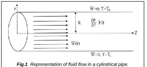
An infinitely long cylinder is considered with the steady incompressible flow of a third grade fluid as can be seen in Figure 1.
The equations for the velocity and the temperature, given by Massoudi and Christe [16] as well as Yurusoy and Pakdemirli [23], may be extended to incorporate a source term (Olajuwon, [18]) and further extended to incorporate a magnetic effect term and a joule heating term, and given by
r
p
r
d
d
r
r
d
d
r
2 2 1)
2
(
1
(1)
p
0
(2)z p r d d r r d d r r d d r r d d r
2
0 3 3 2 ( 1
1 (3)
02
1 2 2
0 0 4 3 2 T T C Q r d d r d d r d T d r r d d r K (4)
The required boundary conditions to solve equations (3) and (4) are
0
)
(
)
(
R
T
R
,(
0
)
(
0
)
0
r
d
T
d
r
d
d
(5)where all symbols are defined in the Nomenclature. The
source term Q represents the heat generation when Q0 and
the heat absorption term when Q 0. The term 02is the magnetic effect term while the term 022 is the joule heating term. Here equation (3) is to be integrated for a given z
p
and once the flow field is determined, the actual pressure field can be obtained from equation (1) and (3). Equation (3) is called the momentum equation while equation (4) is called the energy equation. The corresponding dimensionless equations for equations (3)-(5) are given as the following:
C H dr d r dr d dr d r dr d r dr d r dr d dr
d
2 2 2 2 2
3 (6)
0 1 2 2 2 2 2
J dr d dr d dr d r drd (7)
with boundary conditions
0
)
1
(
)
1
(
, (0) (0)0 dr d drd
, (8)The form of equations (6) and (7) depends on the viscosity model, and the viscosity is assumed to be a function of temperature. We now present the Vogel’s model case as can be found in Massoudi and Christe [31], Pakdemirli and Yilmas [19] and Okoya [17].
Here,
)
(
exp
)
(
0 0T
b
a
T
(9)The corresponding non-dimensional form of equation (9) is
0)
(
exp
T
B
A
(10)The coupled nonlinear ordinary differential equations (6) and (7), with the boundary conditions (8), can be solved in principle by several methods, the Adomian decomposition method being a convenient and effective tool. Here, we shall use the Adomian decomposition method to determine the flow field and thermal distribution.
3 A
NALYTICALS
OLUTIONSIn this section, the Adomian decomposition method series solution will be obtained for the dimensionless velocity and temperature by using the Vogel’s model viscosity. Taking the Maclaurin’s series expansion of the exponential term, we can express equation (10) as
1
(
)
)
(
exp
0
2
2
O
B
A
T
B
A
(11)Which can be written as
*1
2B
A
C
C
(12)
Where
0 *)
(
exp
T
B
A
C
C
This implies that
2 * 11
B
A
C
C
(13)We can write equation (6) as
20 IJSTR©2018 www.ijstr.org 3 1 1 2 2
1
dr
d
r
dr
d
dr
d
dr
d
r
dr
d
1 1 2 2 2 1
3
H
C
dr
d
dr
d
(14)
With the operator 2 2
dr d L
and dr d R
, applying the inverse operator
drdr L1 ()
to both sides of equation (14) and (7) we have equation (15) and (16) respectively
)
(
1
)
(
1
1 1
1
1
R
L
R
R
r
L
CL
Br
A
r
3
(
)
1
1 3 1 1 2 1 11
R
L
R
L
HL
r
L
(15)
R
r
L
JL
L
Er
C
r
)
1
(
1
1 2
1
2
2
R
R
(16)Assuming solutions of the form
0)
(
n nr
(17)
0)
(
n mr
(18)Substituting the series solutions (17) - (18) into equations (11) - (16) and making a one-to-one correspondence between the contributions on the LHS and the terms on the RHS, we obtain the following three point approximations for the velocity and temperature profile as
3 6 7 * 2 2 8 3 * 2 8 5 * 2 6 2 * 2 4 2 * 2 6 2 * 2 4 * 2 4 2 * 2 2 * 4 * 2 4 4 * 4 4 * 2 2 * ) 0 ( 5 8 6720 1 5040 277 360 1 )) 0 ( ( 24 1 ) 0 ( 360 1 ) 0 ( 24 1 ) 0 ( 24 1 ) 0 ( ) 0 ( 2 1 24 1 ) 0 ( 3 1 3 1 ) 0 ( 2 1 ) 1 ( ) 0 ( C r Hw C B AJr C B r A C B Cr A C B r w AJ C B r AJw C B r A C CB r A HC CB r w A HC C r HC CB r A C C r C B r A C w w w (19) 2 2 8 3 * 2 4 2 8 2 5 * 2 4 8 2 3 * 2 2 8 5 * 2 8 3 * 6 4 * 2 4 * 4 * 2 2 4 * 6 2 * 2 ) 0 ( ) 0 ( 672 1 ) 0 ( )) 0 ( ( 168 1 )) 0 ( ( 1344 1 ) 0 ( 168 1 ) 0 ( 1344 1 25 14 ) 0 ( 12 1 18 1 2 1 ) 0 ( 12 1 120 1 ) 0 ( 2 1 ) 1 ( ) 0 ( B C r w C JAH B C r w C H JA CB r C H JA CB r C JA B r AJH C r C B Cr A C r CC r JA r C Jw r JC r (20)
4 C
OMPUTATIONALR
ESULTS
HOWING THEDIFFERENCE BETWEEN
ADOMIAN
DECOMPOSITION
AND PERTURBATION SOLUTIONSFor the purpose of comparison, the mid plane temperature distribution of the pipe (0)max for the obtained Adomian decomposition method solution (ADM) when HJ0, and the perturbation solution (P) of Jayeoba and Okoya (2012) are tabulated. The difference between the solutions obtained by the two methods is also computed.
TABLE 1:DIFFERENCE BETWEEN THE VALUE OF max(ADM) AND
) ( max P
WHEN T0C1
TABLE 2:DIFFERENCE BETWEEN THE VALUE OF max(ADM) AND )
( max P
WHEN 1
0
T C
TABLE 3:DIFFERENCE BETWEEN THE VALUE OF max(ADM) AND )
( max P
WHEN
AB1TABLE 4:DIFFERENCE BETWEEN THE VALUE OF max(ADM) AND )
( max P
WHEN
A
B
1
A B1
)
(
max
ADM
max(
P
)
DifferenceB A1
)
(
max
ADM
max(
P
)
DifferenceC T01
)
(
max
ADM
max(P) Difference0
T C1
) ( max ADM
21 IJSTR©2018
www.ijstr.org
TABLE 5:DIFFERENCE BETWEEN THE VALUE OF ( )
max ADM
AND
) ( max P
WHEN AT0CB1
TABLE 6:DIFFERENCE BETWEEN THE VALUE OF ( )
max ADM
AND
) ( max P
WHEN AT0CB1
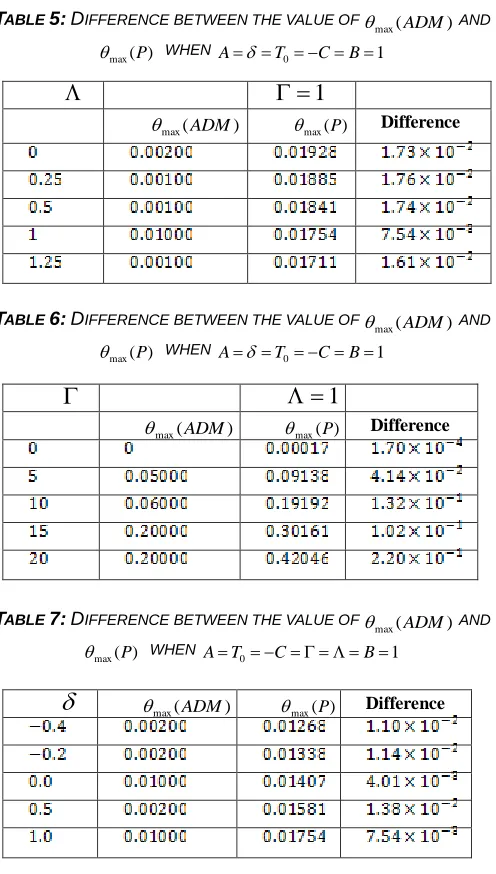
TABLE 7:DIFFERENCE BETWEEN THE VALUE OF max(ADM) AND )
( max P
WHEN AT0CB1
The physical quantities of principle interest according to the Vogel’s model viscosity are
A
,B
andT
0. The difference between the Adomian solution and the perturbation solution asthe values of
A
is varied could be analyzed through Table 1. It is seen from the table that there is a good agreement between the two results as the difference decreases when thevalue of
A
increases. For the variation ofB
in Table 2 the difference is at most1
%
. In Table 3 the variation of thepressure gradient parameter
C
is considered and it is noticed that as the difference increases forC
0
.
25
. ForT
0
0
.
5
the difference is less than
1
%
in Table 4. In Table 5 thedifference as the parameter
is varied is investigated and it is observed that for
1
the difference is at most10
2. Table 6 shows that as
increases the difference increases to at most10
1, which indicates a good agreement between the two results. Finally, the variation of the heat generation/absorption parameter
is shown in Table 7. For1
4
.
0
the results are in good agreement with a thedifference reducing to
0
.
7
%
. From the above data it is clear that the Adomian decomposition method is appropriate for solving the problem presented in this paper. Now that we have established the validity of the Adomian decomposition method, we proceed to capture the effect of the various thermo-physical parameters on the solutions of the momentum and energy equations.5 OUTPUTS AND ANALYSIS
The analytical solutions (19) – (20) for the dimensionless velocity and temperature distributions, for various values of the thermo-physical parameters are plotted against the radius of the pipe. The velocity graphs for the different thermo-physical parameters are represented by Figs. 2 – 10 while the temperature graphs are represented by Figs. 11 – 19. In these figures, the variations of the thermo-physical parameters are taken into account.
1
) ( max ADM
max(P) Difference
1
) ( max ADM
max(P) Difference
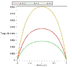
max(ADM) max(P) DifferenceFig. 2.Velocity Graphs for Different Values of the Dimensionless Constant from Vogel’s Viscosity Model
A
with1
0
H J
T CFig. 3.Velocity Graphs for Different Values of the DimensionlessConstant from Vogel’s Viscosity Model B with
1 0
H J T C
Fig. 4.Velocity Graphs for Different Values of the Pressure Gradient Parameter
C
with1 0
22 IJSTR©2018
www.ijstr.org
Fig. 5.Velocity Graphs for Different Values of the Initial
TemperatureT0with
H
J
A
B
C
1
Fig. 6. Velocity Graphs for Different Values of the Non-Newtonian Parameter
with
H
J
A
B
T
0
C
1
Fig. 7. Velocity Graphs for Different Values of the Viscous Dissipation Parameter
withHJ ABT0 C1
Fig. 8. Velocity Graphs for Different Values of the Heat Generation Parameterwith H JABT0C1
Fig. 9. Velocity Graphs for Different Values of the Magnetic Effect Parameter H with
J ABT0C1Fig. 10. Velocity Graphs for Different Values of the Joule Heating Parameter J with H
ABT0C 1Fig. 11. Temperature Graphs for Different Values of the Dimensionless Constant from Vogel’s Viscosity Model
A
23 IJSTR©2018
www.ijstr.org
Fig. 12.Temperature Graphs for Different Values of the Dimensionless Constant from Vogel’s Viscosity Model B with
1 0
H J
T CFig. 13. Temperature Graphs for Different Values of the Pressure Gradient Parameter Cwith HJ T0 AB1
Fig. 14. Temperature Graphs for Different Values of the Initial Temperature
T
0 with HJ ABC1Fig. 15. Temperature Graphs for Different Values of the
Non-Newtonian Parameter with 1
0
H J A B T C
Fig. 16. Temperature Graphs for Different Values of the Viscous Dissipation Parameter with 1
0
H J A B T C
Fig. 17. Temperature Graphs for Different Values of the Heat Generation Parameter
with HJABT0C1Fig. 18. Temperature Graphs for Different Values of the Magnetic
Effect Parameter H with 1
0
24 IJSTR©2018
www.ijstr.org Figures 2 and 11 are the velocity and temperature profiles for various values of the dimensionless constant from Vogel’s viscosity model A, when the values of the other thermo-physical parameters are equal to one (1), respectively. In Figures 2 and 11 the maximum velocity occurs at the point
0
r
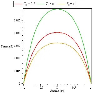
which is the middle of the pipe. As the values of A increases the velocity and temperature of the fluid reduces. Figures 3 and 12 reveal the effect of the dimensionless constant from Vogel’s viscosity model B on the velocity and temperature profiles respectively. As the values of B increases there is a corresponding increase in both the velocity and temperature of the fluid. The behaviour of the velocity and temperature of the fluid as the pressure gradient parameter Cis varied is captured in Figures 4 and 13 respectively. As thevalue of C drops from 0.5 to 1 there is a steady increase in both the velocity and temperature. Figure 5 and 14 presents the effect of the Initial Temperature
T
0 on the velocity and temperature profiles respectively. Increase in the Initial Temperature T0 leads to a reduction in both the velocity and temperature of the fluid as can be seen. Influence of the non-Newtonian material parameter of the fluid on the velocity and temperature profiles is shown in Figures 6 and 15 respectively. In Figure 6, it is observed that as the value of increases the maximum velocity at the middle of the pipe decreases. Increase in the value of results in an increase in the maximum temperature of the fluid at the middle of the pipe, as can be seen in Figure 15. The case when 0 corresponds to a Newtonian fluid. The velocity and temperature distribution for various values of the viscous dissipation parameter is presented in Figures 7 and 16 respectively. Increase in values of tends to increase the velocity as seen in Figure 7. Also, in Figure 16 increase in the value of appears to increase the temperature of the fluid due to the irreversible conversion of mechanical energy to thermal energy. This holds true for this study as well as for the study by Jayeoba and Okoya (2012) and previous ones. The effect of the heat generation parameter
on the velocity and temperature is shown in Figures 8 and 17 respectively. These figures indicate that as the value of
increases the velocity and temperature of the fluid also increases. The influence of various values of the magnetic effect parameter H on the dimensionless velocity and temperature is depicted by Figures 9 and 18 respectively. In Figure 9 increment in the value ofH
brings about a steady increase in the velocity of the fluid. While in Figure 12 it is evident that increase in the value of the magnetic effect parameter only brings about a gradual increase the temperature of the fluid. Figures 10 and 19 portray the effect of the joule heating parameter
J
on the velocity and temperature of the fluid respectively. As the value ofJ
increases the velocity increases as well as the temperature of the fluid. WhenJ
is relatively large the fluid finally exceeds the least temperature distribution.6 CONCLUSION
In this paper we extended the model equations of Olajuwon (2009) by incorporating a magnetic effect term in the momentum equation and a joule heating term in the energy equation. This extension of ours gave rise to a magnetohydrodynamic flow problem of a third grade fluid through a cylindrical pipe. We converted the dimensional momentum and energy equations to dimensionless equations and used the Adomian decomposition method for the Vogel’s viscosity model to develop a recurrence algorithm. A three point approximate analytical solution to the velocity and temperature was obtained using the computer software Mapple (13). The results for various values of the thermo-physical parameters were presented in graphs, from which we make the following conclusions: Increase in dimensionless constant from Vogel’s viscosity model A brings about a decrease in both the velocity and the temperature, while increase in the dimensionless constant from Vogel’s viscosity model
B
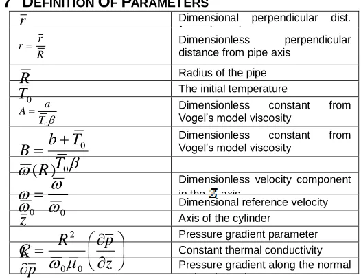
results in an increase in both the velocity and temperature of the fluid. The more negative the value of the pressure gradient parameter becomes, the higher the velocity and temperature of the fluid. Increase in the initial temperature reduces the velocity and temperature of the fluid, this is as a result of the presence of joule heating. Increase in the non-Newtonian material parameter of the fluid decreases the velocity and increases the temperature of the fluid. Increase in the viscous dissipation parameter increases both the velocity and temperature of the fluid. The heat generation parameter increases the velocity and temperature of the fluid. The magnetic effect parameter increases the velocity of the fluid as well as its temperature. Increases in the joule heating parameter results in the increase in both the velocity and temperature of the fluid.7 DEFINITION OF PARAMETERS
r
Dimensional perpendicular dist.from pipe axis
R r
r Dimensionless perpendicular
distance from pipe axis
R
Radius of the pipe0
T
The initial temperature 0
T a
A Dimensionless Vogel’s model viscosity constant from
0 0
T
T
b
B
Dimensionless constant from Vogel’s model viscosity
)
(
R
0
Dimensionless velocity component in the axis 0
Dimensional reference velocityz
Axis of the cylinder
z
p
R
C
0 0
2
Pressure gradient parameter
K
Constant thermal conductivityr
p
Pressure gradient along the normalto the pipe axis
25 IJSTR©2018
www.ijstr.org
z
p
Pressure gradient in the axialdirection
p
Pressure gradient in rotational directionQ
Heat generation constant0
C
Initial concentration of the reactant speciesGreek symbols
3 2 1
,
,
Constant materialcoefficients
E T R 0
Activation energy
0
T M
Reynold’s ViscosityVariational Parameter
Dynamic shear viscositye
0
,)
exp(
0 00
0
T
e
Dimensionless viscosity
Rotational direction
2 0
0
T
R
E
T
T
Dimensionlesstemperature excess
0 2 0 0
4
T
e
Viscous heatingparameter
2 0 0
2 0 3
r
Non-Newtonian materialparameter of the fluid
2 0
0 2 0
T
KR
C
R
EA
Q
Heat generationparameter
0 2 0 2
RH Magnetic Parameter Effect
2 0
2 0 2 0 2
T
KR
R
E
J
Joule Heating ParameterREFERENCES
[1] G. A. Adomian, ―A Review of the Decomposition Method and some Results for Non-linear Equation,‖ Mathematics and Computer Modelling, vol. 13, no. 7, pp. 17-43, 1992.
[2] G. A. Adomian, Solving Frontier Problems of Physics: The Decomposition Method, Volume 60. Dordrecht, Kluwer Academic Publishers. 370pp.
[3] Y. M. Aiyesimi, G. T. Okedayo, and O. W. Lawal, ―MHD Flow of a Third Grade Fluid with Heat Transfer and Slip Boundary Condition down an Inclined Plane,‖ Mathematical Theory and Modeling, vol. 2, no. 9, pp. 108-120, 2012a.
[4] Y. M. Aiyesimi, S. O. Abah, and G. T. Okedayo, ―Radiative Effects on the Unsteady Double Diffusive MHD Boundary Layer Flow over a Stretching Vertical Plate,‖ American Journal of Scientific Research , vol. 65, pp. 51-61, 2012b.
[5] H. Alfvn, ―Existence of Electromagnetic-hydrodynamic Wave,‖ Nature, vol. 150, pp. 405-406, 1942.
[6] H. Branover, and P. Gershon, ―MHD Turbulence Study,‖ Report BGUN-RDA-100-176. Ben-Gurion University, 1976.
[7] T. De, S. Costa, and D. Sandberg, ―Mathematical Model of a Smoldering Log,‖ Combustion and Flame, vol. 139, pp. 227-238, 2004.
[8] J. A. Gbadeyan, A. S. Idowu, G. T. Okedayo, L. O. Ahmed, and O. W. Lawal, ―Effect of Suction on Thin Film Flow of a Third Grade Fluid in a Porous Medium down an Inclined Plane with Heat Transfer,‖ International Journal of Scientific and Engineering Research, vol. 5, no. 4, pp. 748-754, 2014.
[9] J. I. Hartmann, ―Hydrodynamics, Theory of Laminar Flow of an Electrically Conducting Liquid in a Homogeneous
Magnetic Field,‖ International
KongeligeDanskeVidenskabernesSelskabMatematisk-FysiskeMeddelelser, vol. 15, pp. 1-27, 1937.
[10] T. Hayat, A. Shafiq, and A. Alsaedi, ―Effect of Joule Heating and Thermal Radiation in Flow of Third Grade Fluid over Radiative Surface,‖ Public Library of Science (PLoS One), vol. 9, no. 1, pp. 133-153, 2014.
[11] R. J. Holroyd, ―An Experimental Study of the Effect of Wall Conductivity, Non-uniform Magnetic Field and Variable-area Ducts on Liquid Metal Flow at High Hartmann Number, Part 1: Ducts with Non-conducting Wall,‖ Journal of Fluid Mechanics, vol. 93, pp. 609-630, 1979.
[12] R. J. Holroyd, ―MHD Flow in a Rectangular Duct with Pairs of Conducting and Non-conducting Walls in the Presence of a Non-uniform Magnetic Field,‖ Journal of Fluid Mechanics, vol. 96, pp. 335-342, 1980.
[13] M. O. Iyoko, G. T. Okedayo, T. Aboiyar, and L. N. Ikpakyegh, ―MHD Flow of a Third Grade Fluid in a Cylindrical Pipe in the presence of Reynolds’ Model Viscosity and Joule Heating,‖ FUW Trends in Science and Technology Journal, vol. 2, no. 1B, pp. 514-520, 2017.
[14] O. J. Jayeoba, and S. S. Okoya, ―Approximate Analytical Solutions for Pipe Flow of a Third Grade Fluid with Variable Models of Viscosities and Heat Generation/Absorption,‖ Journal of Nigerian Mathematical Society, vol. 31, pp. 207-227, 2012.
[15] O. D. Makinde, ―Hermite- Pade Approach to Thermal Radiation Effect on Inherent Irreversibility in a Variable Viscosity Channel Flow,‖ Computers and Mathematics with Applications, vol. 58, pp. 2330-2338, 2009.
26 IJSTR©2018
www.ijstr.org and Viscous Dissipation on the Flow of Third Grade Fluid in a Pipe,‖ International Journal of Non-linear Mechanics, vol. 30, no. 5, pp. 687-699, 1996.
[17] S. S. Okoya, ―Disappearance of Criticality for Reactive Third Grade Fluid with Reynold’s Model Viscosity in a Flat Channel,‖.International Journal of Non-linear Mechanics, vol. 46, no. 9, pp. 1110-1111, 2011.
[18] B. I. Olajuwon, ―Flow and Natural Convection Heat Transfer in a Power Law Fluid past a Vertical Plate with Heat Generation,‖ International Journal of Non-linear Science, vol. 7, no. 1, pp. 50-56,2009.
[19] M. Pakdemirli, and B. S. Yilbas, ― Entropy Generation for Pipe Flow of a Third Grade Fluid with Vogel Model Viscosity,‖ International Journal of Non-linear Mechanics,vol. 41, no. 3, pp. 432-437, 2006.
[20] B. Raftari, F. Parvaneh, and K. Vajravelu, ―Homotopy Analysis of the Magnetohydrodynamic Flow and Heat Transfer of a Second Grade Fluid in a Porous Channel,‖ Energy, vol. 59, pp. 625-632, 2013.
[21] A. M. Siddiqui, M. Hameed, B. M. Siddiqui, and Q. K. Ghori, ―Use of Adomoian Decomposition Method in the Study of Parrallel Plate Flow of a Third Grade Fluid,‖ International Journal of Non-linear Mechanics, vol. 40, pp. 807-820, 2005.
[22] P. Smith, ―Some AsymtoticExtremum Principle for Magnetohydrodynamic Pipe Flow,‖ Applied Science Resources, vol.24, pp. 452-466, 1971.
[23] M. Yurusoy, and M. Pakdemirli, ―Approximate Analytical Solution for the Flow of a Third Grade Fluid in a Pipe,‖ International Journal of Non-linear Mechanics, vol. 37, no. 2, pp. 187-195, 2002.
[24] C. Y. Tsai, , M. Novack and G, Roffle, ―Rheological and Heat Transfer Characteristics of Flowing Coal-Water Mixtures,‖ Final Report, DOE/MC, pp. 2325-2763, 1988.
[25] B. Raftari, and A. Yildirim, ―Series Solution of a Nonlinear ODE arising in Magnetohydrodynamics by HPM-Pad Technique,‖ Computer and Mathematics Applications, vol. 61, pp. 1676-1681, 2011a.
[26] B. Raftari, and A. Yildirim, ―A New Modified Homotpy Perturbation Method with Two Free Auxiliary Parameters for Solving MHD Viscous Flow due to a Shrinking Sheet,‖ Engineering Computations, vol. 28, no. 5, pp. 528-539, 2011b.
[27] B. Raftari, S. T. Mohyud-Din, and A. Yildirim, ―Solution to the MHD Flow over a Non-linear Stretching Sheet by Homotopy Perturbation Method,‖ SCIENCE CHINA Physics and Mechanical Astronomy, vol. 54, no. 2, pp. 342-345, 2011.
[28] B. Raftari, and A. Yildirim, ―Homotpy Perturbation Method for Heat and Mass Transfer in Magnetohydrodynamic Flow,‖ Journal of Thermophysics and Heat Transfer, vol.
26, no. 1, pp. 154-160, 2012.
[29] B. Raftari, and K. Vajravelu, ―Homotpy Analysis Method for MHD Viscoelastic Fluid Flow and Heat Transfer in a Channel with Stretching Wall,‖ Communications in Nonlinear Science and Numerical Simulation, vol. 17, pp. 4149-4162, 2012.
[30] B. Raftari, and A. Yildirim, ―The Application of Homotpy Perturbation Method for MHD Flow of UCM Fluids above Porous Stretching Sheets,‖ Computer and Mathematics Applications, vol. 59, pp. 3328-3337, 2010.