OPTIMAL POWER FLOW AND LOAD FLOW ANALYSIS WITH CONSIDERING DIFFERENT DG INTEGRATION RATES

Optimal Power Flow and Load Flow Analysis with Considering Different DG

Integration Rates

Mehmet Şefik Üney

, Halil Çimen

, Nurettin Çetinkaya

and Mehmet Latif Levent

1_{Department of Electrical and Electronics Engineering, Şırnak University, Şırnak, Turkey.} 2

Department of Electrical and Electronics Engineering, Selçuk University, Konya, Turkey.

3

Department of Electrical and Electronics Engineering, Hakkâri University, Hakkâri, Turkey.

Article Received: 15 August 2017 Article Accepted: 30 November 2017 Article Published: 30 December 2017

1. INTRODUCTION

Optimal Power Flow was first introduced in the 1960s [1] and still remains to be a fundamental optimization problem in electrical power systems analysis. There are two challenges in the solution of OPF. First, it is an

operational level problem solved every few minutes, hence the computational budget is limited. Second, it is a non-convex optimization problem on a large-scale power network of thousands of buses, generators, and loads.

The importance of the problem and the aforementioned difficulties have produced a rich literature. Commonly used analysis model in power system is load flow analysis. The calculation of the load flow in the transmission

lines and the transformers is called load flow analysis. It is necessary that not overloading of transmission lines and transformers in power systems, the voltages remain within certain limits for all buses and generator's reactive

production to remain within acceptable limits.

Most commonly used iterative methods in solving power flow and load flow problems are the Newton-Raphson

(N-R), the Gauss-Seidel, and the Fast -Decoupled method [2]. N-R method is used in this work because it is more reliable and converges faster with minimum iterations [3]. But these techniques are not suitable for systems

having complex non-convex, non-smooth, and non-differentiable objective functions and constraints. Many heuristic algorithms have been projected to address the problem for solving load flow and non linear optimal

power flow problems, such as evolutionary programming (EP)[4], genetic algorithm (GA) [5], hybrid evolutionary programming (HEP) [6], particle swarm optimization (PSO) [7], differential evolution (DE) [8], tabu

search [9], chaotic ant swarm optimization (CASO) [10], biogeography-based optimization (BBO) [11], bacteria foraging optimization (BFO) [12], harmony search algorithm (HSA) [13], gravitational search algorithm (GSA)

[14], teaching learning based algorithm (TLBO) [16], etc. and their effectiveness have been established.

A B S T R A C T

Lately, there is an increasing need for Optimal Power Flow (OPF) to solve problems of today’s regulated and deregulated power systems and the unsolved problems in the vertically integrated power systems. The objective of an optimal power flow is to determine the best way to instantaneously operate a power system. OPF is considered with the goal of limiting either the power circulation misfortunes or the cost of influence drawn from the substation and provided by distributed generation (DG) units. The most important aspects related to OPF are the solution methodologies and the application areas. This paper presents OPF and load flow analysis of IEEE 30 bus system with DG. PV plant is determined as DG plant. According to different PV integration rates, system parameters are analysed. Especially active and reactive losses are investigated. More than 30% PV contribution in transmission and distribution systems can affect the system adversely. Because of this reason, the PV contribution limit is set at 30%. Newton-Raphson method is used as the load flow analysis method.

2.PROBLEMFORMULATION

Mathematically, an OPF problem can be formulated as follows:

min f(x, u) (The objective function) (1)

subject to g(x, u) = 0 (Equality constraints) (2)

(x, u) 0

h  (Inequality constraints) (3)

Where;

x the vector of dependent variables consisting of slack bus power Pg1, load bus voltage vector VL, generator

reactive power output Q_g, and transmission line loading vector S_l.

uthe vector of independent variables consisting of generators voltage magnitude vector V_g, generator real power

output vector P_g except slack bus real power output P_g1, transformer tap settings vector T, and settings of the shunt

VAR compensation vector Q_c.

Hence;

T

g1 L g l

x

=



_



_

=

_





_

The equality constraints h(x, u) represent typical load flow equations [17, 18]. The inequality constraints g(x, u)

represent the system operating constraints which can be arranged as follows:

 Generator maximum and minimum real and reactive powers:

min max

g g g

P P P (5)

min max

g g g

Q Q Q (6)

 Maximum and minimum tap ratio of under-load tap changing transformers:

min max

T

 

 Maximum and minimum limits of shunt VAR compensators

min max

c c c

Q





 Maximum and minimum of bus voltage magnitudes and line flows to maintain the quality of electrical

service and system security:

min max

L L L

V





min max

g g g

V V V (10)

2 2 _max

3.APPLICATION

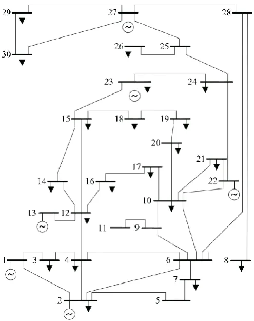
FIGURE 1 SHOWS THE IEEE-30 BUS TEST SYSTEM. IN ADDITION, INPUT DATA OF THE TEST SYSTEM WHICH ARE

GIVEN IN TABLE 3, TABLE 4 AND TABLE 5 DEFINED IN APPENDIX

Figure 1. IEEE-30 bus test system

Optimal Power Flow system solves power system load flow, optimizes system operating conditions, and adjusts

control variable settings, while ensuring system constraints are not violated. An optimized system will reduce the installation and/or operating cost, improve overall system performance, and increase its reliability and security. It is

also provides a variety of other choices of optimization objectives, which covers virtually all the optimization criteria for a real power system. Any practical control methods in a power system are considered in the calculation.

Constraints for bus voltage, branch flow in different types (MVA, MW, Mvar, and Amp), as well as control variable adjustable bounds are also available for users to select and utilize.

The Load Flow Analysis can create and validate system models and obtain accurate and reliable results. It can calculate bus voltages, branch power factors, currents, and power flows throughout the electrical system. Load

flow also allows for swing, voltage regulated, and unregulated power sources with multiple power grids and generator connections. It is also capable of performing analysis on both radial and loop systems and has an option

The number of iterations for Optimal Power Flow system is 11 and for Load Flow Analysis is 3. The system frequency is assumed to be 50 Hz. Bus 1 is considered to be the swing bus. The bus input data, line/cable data,

generator data and branch connections are input to the system with reference to the Alsac O. & Stott B, "Optimal Load Flow with Steady State Security". Electrical loads those are active during normal power operation mode of

plant are identified and their breaker are set to closed state. Voltage ratings, power rating, impedances, RPMs etc., are entered into load data, generator and transformer data. The Summary of total generation, loading & demand is

shown in Table 1 and Table 2.

Table 1. Power Flow Summary

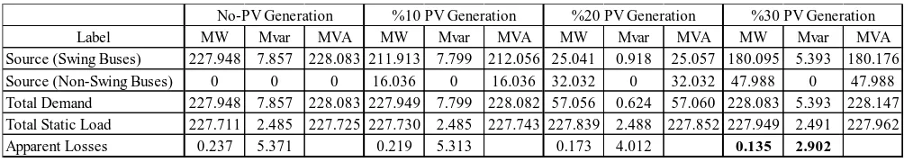
Table 2. Load Flow Summary

Optimum power flow and load flow analysis results are seen in the tables above. First, the optimum power flow

results are examined. Different production values of the PV plant are taken into account. These values are No-PV, 10%, 20% and 30%. When the results are examined, it is seen that 10% PV production has no significant effect on

the system. Active losses in 20% production are minimum. However, reactive losses are minimum in 30% production. According to these values, active and reactive power losses are minimized at different production

values. Secondly, the results of load flow analysis are examined. When these results are examined, it is seen that losses decrease as PV production increases. It is seen that active and reactive losses are minimum in 30%

production. More than 30% PV contribution in transmission and distribution systems can make the system unbalanced. The reason of this is PV production is variable. Production is constantly changing due to weather conditions. This variability can adversely affect the system. For this reason, the PV contribution limit is set at 30%.

In order to study more PV contribution, it is necessary to consider the system balance.

4. CONCLUSION

In this work, optimum power flow and load flow problems are solved for the IEEE-30 bus test system.

Meta-heuristic algorithms were used to solve the problem of optimum power flow. For load flow analysis,

Label MW Mvar MVA MW Mvar MVA MW Mvar MVA MW Mvar MVA Source (Swing Buses) 40.978 1.921 41.023 41.360 1.922 41.405 25.041 0.918 25.057 15.627 0.772 15.646

Source (Non-Swing Buses) 0 0 0 0 0 0 0 0 0 0 0 0

Total Demand 56.969 0.622 56.972 56.969 0.622 56.972 57.056 0.624 57.060 62.547 0.696 62.550 Apparent Losses 0.046 1.299 0.046 1.300 0.017 0.294 0.044 0.086

No-PV Generation %10 PV Generation %20 PV Generation %30 PV Generation

Label MW Mvar MVA MW Mvar MVA MW Mvar MVA MW Mvar MVA Source (Swing Buses) 227.948 7.857 228.083 211.913 7.799 212.056 25.041 0.918 25.057 180.095 5.393 180.176 Source (Non-Swing Buses) 0 0 0 16.036 0 16.036 32.032 0 32.032 47.988 0 47.988 Total Demand 227.948 7.857 228.083 227.949 7.799 228.082 57.056 0.624 57.060 228.083 5.393 228.147 Total Static Load 227.711 2.485 227.725 227.730 2.485 227.743 227.839 2.488 227.852 227.949 2.491 227.962 Apparent Losses 0.237 5.371 0.219 5.313 0.173 4.012 0.135 2.902

No-PV, 10%, 20% and 30% generation rates were added to the system. Firstly, when the optimum power flow results are examined, it is seen that 10% PV production has no significant effect on the system. Active losses in

20% production are minimum. However, reactive losses are minimum in 30% production. According to these values, active and reactive power losses are minimized at different production values. Secondly, when the results of

load flow analysis are examined, it is seen that losses decrease as PV production increases. It is seen that active and reactive losses are minimum in 30% production. Furthermore, more than 30% PV contribution in transmission and

distribution systems can make the system unbalanced. The reason of this is PV generation is variable. Generation is constantly changing due to weather conditions. This variability can adversely affect the system. For this reason, the

PV contribution limit is set at 30%. In order to study more PV contribution, it is necessary to consider the system balance.

REFERENCES

[1] Carpentier, J., “Contributions to the economic dispatch problem,” Bulletin Society Francaise Electriciens, vol. 8, no. 3, pp. 431{447, 1962.

[2] Keyhani, A., Abur, A. and Hao, S., “Evaluation of Power Flow Techniques for Personal Computers,” IEEE

Transactions on Power Systems, 4, 817-826,1989.

[3] Afolabi, O.A., Ali, W.H., Cofie, P., Fuller, J., Obiomon, P. andKolawole, E.S., “Analysis of the Load Flow Problem in Power System Planning Studies,” Energy and Power Engineering, 7, 509-523, 2015.

[4] J. Yuryevich and Kit Po Wong, "Evolutionary programming based optimal power flow algorithm," 1999 IEEE Power Engineering Societ Summer Meeting. Conference Proceedings (Cat. No.99CH36364), Edmonton, Alta.,

1999, pp. 1267 vol.2-. doi: 10.1109/PESS.1999.787503.

[5] L.L. Lai, J.T. Ma, R. Yokoyama, M. Zhao, Improved genetic algorithms for optimal power flow under both normal and contingent operation states, International Journal of Electrical Power & Energy Systems, Volume 19,

Issue 5, 1997, Pages 287-292, ISSN 0142-0615, http://dx.doi.org/10.1016/S0142-0615(96)00051-8.

[6] A. K. Swain and A. S. Morris, "A novel hybrid evolutionary programming method for function optimization,"

Proceedings of the 2000 Congress on Evolutionary Computation. CEC00 (Cat. No.00TH8512), La Jolla, CA, 2000, pp. 699-705 vol.1. doi: 10.1109/CEC.2000.870366.

[7] M.A. Abido, Optimal power flow using particle swarm optimization, International Journal of Electrical Power

[8] A.A. Abou El Ela, M.A. Abido, S.R. Spea, Optimal power flow using differential evolution algorithm, Electric Power Systems Research, Volume 80, Issue 7, July 2010, Pages 878-885, ISSN 0378-7796,

http://dx.doi.org/10.1016/j.epsr.2009.12.018.

[9] M.A. Abido, Optimal power flow using tabu search algorithm, Electr. Power Comp. Syst. 30 (5) (2002) 469– 483.

[10] Jiejin Cai, Xiaoqian Ma, Lixiang Li, Yixian Yang, Haipeng Peng, Xiangdong Wang, Chaotic ant swarm

optimization to economic dispatch, Electric Power Systems Research, Volume 77, Issue 10, August 2007, Pages 1373-1380, ISSN 0378-7796, http://dx.doi.org/10.1016/j.epsr.2006.10.006.

[11] P.K. Roy, S.P. Ghoshal, S.S. Thakur, Biogeography based optimization for multi-constraint optimal power

flow with emission and non-smooth cost function, Expert Systems with Applications, Volume 37, Issue 12, December 2010, Pages 8221-8228, ISSN 0957-4174, http://dx.doi.org/10.1016/j.eswa.2010.05.064.

[12] M. Tripathy and S. Mishra, "Bacteria Foraging-Based Solution to Optimize Both Real Power Loss and Voltage Stability Limit," in IEEE Transactions on Power Systems, vol. 22, no. 1, pp. 240-248, Feb. 2007. doi:

10.1109/TPWRS.2006.887968.

[13] A.H. Khazali, M. Kalantar, Optimal reactive power dispatch based on harmony search algorithm, International Journal of Electrical Power & Energy Systems, Volume 33, Issue 3, March 2011, Pages 684-692, ISSN 0142-0615,

http://dx.doi.org/10.1016/j.ijepes.2010.11.018.

[14] P. K. Roy, B. Mandal, & K. Bhattacharya, (2012). Gravitational search algorithm based optimal reactive power dispatch for voltage stability enhancement. Electric Power Components and Systems, 40(9), 956-976.

[15] M. A. Abido, (2011). Multiobjective particle swarm optimization for optimal power flow problem. In

Handbook of swarm intelligence (pp. 241-268). Springer Berlin Heidelberg.

[16] M. Basu, (2014). Teaching–learning-based optimization algorithm for multi-area economic dispatch. Energy,

68, 21-28.

[17] John J. Grainger, William D. Stevenson,” Power System analysis”, McGraw Hill Inc., 1994.

APPENDİX

Table 3. IEEE 30 Bus Data

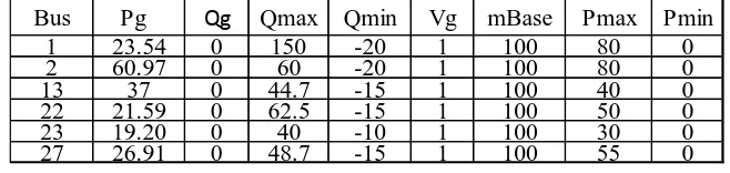
TABLE 4. IEEE 30 GENERATOR DATA

Bus Type Pd Qd Gs Bs Area Vm Va BaseKV Vmax Vmin

1 3 0 0 0 0 1 1 135 1 42856 0.95

2 2 42937 42928 0 0 1 1 135 1 42736 0.95

3 1 42827 42767 0 0 1 1 135 1 42856 0.95

4 1 42893 42887 0 0 1 1 135 1 42856 0.95

5 1 0 0 0 0.19 1 1 135 1 42856 0.95

6 1 0 0 0 0 1 1 135 1 42856 0.95

7 1 42969 42988 0 0 1 1 135 1 42856 0.95

8 1 30 30 0 0 1 1 135 1 42856 0.95

9 1 0 0 0 0 1 1 135 1 42856 0.95

10 1 42952 2 0 0 3 1 135 1 42856 0.95

11 1 0 0 0 0 1 1 135 1 42856 0.95

12 1 42777 42862 0 0 2 1 135 1 42856 0.95

13 2 0 0 0 0 2 1 135 1 42736 0.95

14 1 42772 42887 0 0 2 1 135 1 42856 0.95

15 1 42774 42857 0 0 2 1 135 1 42856 0.95

16 1 42858 42948 0 0 2 1 135 1 42856 0.95

17 1 9 42952 0 0 2 1 135 1 42856 0.95

18 1 42769 0.9 0 0 2 1 135 1 42856 0.95

19 1 42864 42828 0 0 2 1 135 1 42856 0.95

20 1 42768 0.7 0 0 2 1 135 1 42856 0.95

21 1 42872 42777 0 0 3 1 135 1 42856 0.95

22 2 0 0 0 0 3 1 135 1 42736 0.95

23 2 42769 42887 0 0 2 1 135 1 42736 0.95

24 1 42924 42922 0 0.04 3 1 135 1 42856 0.95

25 1 0 0 0 0 3 1 135 1 42856 0.95

26 1 42858 42796 0 0 3 1 135 1 42856 0.95

27 2 0 0 0 0 3 1 135 1 42736 0.95

28 1 0 0 0 0 1 1 135 1 42856 0.95

29 1 42827 0.9 0 0 3 1 135 1 42856 0.95

30 1 42896 42979 0 0 3 1 135 1 42856 0.95

Bus Pg Qg Qmax Qmin Vg mBase Pmax Pmin

1 23.54 0 150 -20 1 100 80 0

2 60.97 0 60 -20 1 100 80 0

13 37 0 44.7 -15 1 100 40 0

22 21.59 0 62.5 -15 1 100 50 0

23 19.20 0 40 -10 1 100 30 0

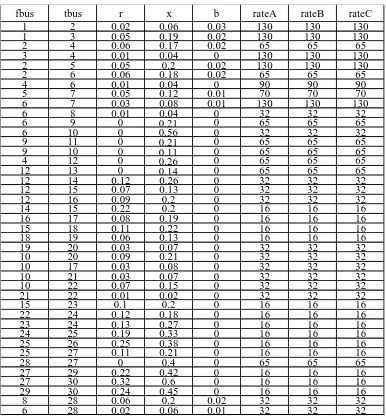
Table 5. IEEE 30 Branch Data

fbus tbus r x b rateA rateB rateC

1 2 0.02 0.06 0.03 130 130 130

1 3 0.05 0.19 0.02 130 130 130

2 4 0.06 0.17 0.02 65 65 65

3 4 0.01 0.04 0 130 130 130

2 5 0.05 0.2 0.02 130 130 130

2 6 0.06 0.18 0.02 65 65 65

4 6 0.01 0.04 0 90 90 90

5 7 0.05 0.12 0.01 70 70 70

6 7 0.03 0.08 0.01 130 130 130

6 8 0.01 0.04 0 32 32 32

6 9 0 0.21 0 65 65 65

6 10 0 0.56 0 32 32 32

9 11 0 0.21 0 65 65 65

9 10 0 0.11 0 65 65 65

4 12 0 0.26 0 65 65 65

12 13 0 0.14 0 65 65 65

12 14 0.12 0.26 0 32 32 32

12 15 0.07 0.13 0 32 32 32

12 16 0.09 0.2 0 32 32 32

14 15 0.22 0.2 0 16 16 16

16 17 0.08 0.19 0 16 16 16

15 18 0.11 0.22 0 16 16 16

18 19 0.06 0.13 0 16 16 16

19 20 0.03 0.07 0 32 32 32

10 20 0.09 0.21 0 32 32 32

10 17 0.03 0.08 0 32 32 32

10 21 0.03 0.07 0 32 32 32

10 22 0.07 0.15 0 32 32 32

21 22 0.01 0.02 0 32 32 32

15 23 0.1 0.2 0 16 16 16

22 24 0.12 0.18 0 16 16 16

23 24 0.13 0.27 0 16 16 16

24 25 0.19 0.33 0 16 16 16

25 26 0.25 0.38 0 16 16 16

25 27 0.11 0.21 0 16 16 16

28 27 0 0.4 0 65 65 65

27 29 0.22 0.42 0 16 16 16

27 30 0.32 0.6 0 16 16 16

29 30 0.24 0.45 0 16 16 16

8 28 0.06 0.2 0.02 32 32 32