Rational Approximation for the one-Dimensional Bratu
Equation
Moustafa Aly Soliman
Chemical Engineering Department, The British University in Egypt El Sherouk City, Cairo, 11837, Egypt
e-mail: [email protected]
Abstract-- The solution of the one dimensional planar Bratu equation is characterized by having two branches. The two branches meet at a limit point that can be obtained through the solution of an eigen-relation. In this paper a transformation is introduced to transform this highly non-linear problem to a linear one. Rational expressions are given for the solution of the Bratu equation and the limit point. This is done using collocation and perturbation techniques.
Index Term
--
Bratu problem, collocation, rational function, perturbation1. INTRODUCTION
Several theoretical studies and numerical methods were used for the study of the Bratu problem [1-6] which models thermal explosion in a slab enclosure. Frank- Kamenetskii [1] formulated the problem and obtained analytical solutions for the case of a slab and cylinder enclosure. The numerical methods used for its solution included the Chebychev pseudospectral method [2] B-splines [3], and variational methods [4]. Mohsen [5] used Green’s function and the resulting integral equation was discretized and the non-linear equations formed are solved. For more references on the subject, one can refer to references [2,5].
The Bratu problem is given by
0
)
exp(
2 2
u
dx
u
d
(1)
0
)
1
(
u
(2)0
)
0
(
dx
du
(3)
There is a critical value for the Frank-Kamenetskii parameter
above which there is no solution to the Bratu problem.Below this value there are two solutions. Harley and Momoniat [6] have shown how the Frank-Kamenetskii parameter can be obtained in terms of the first integrals.
This problem has the analytical solution given by
))
2
/
(
sec
log(
)
,
(
x
z
2h
2z
x
u
(4)Where z is the solution of the eigen-relation
)
2
/
cosh(
z
z
(5)Boyd [2] recently obtained approximate relations for this equation. He also showed that much information about the solution of the one-dimensional Bratu equation can be obtained by applying one point collocation. The choice of the collocation points depend on what points we need the solution to be accurate at.
For the linear boundary value problem
0
)
1
(
2 2
u
dx
u
d
(6)
0
)
1
(
u
(7)0
)
0
(
dx
du
(8)
The choice of the collocation points as the zeros of Jacobi
polynomials with a weight of
(
1
x
2)
[7-9] will ensure thatthe solution is correct to the order of
n1 at the collocationpoints and to the order of
n elsewhere where n is thepolynomial order. We call this method “standard collocation method” [7-9].The integral
1
0
udx
I
(9)will be correct to the order of
n1In one point collocation, the collocation point at which the
solution is valid up to the order of λ2, is
44721
.
0
5
/
1
1
x
(10)If we would like the solution to be correct to the order of
24082483
.
0
6
/
1
1
x
(11)This explains why the choice of
4030414705
.
0
1
x
(12)made by Boyd [2] to obtain accurate prediction of the limit point λ = 0.8784576797812903015. At this point z=1.81017 and u(0)=1.18684.
In this paper we first obtain an approximate solution to the eigen- relation (5) then we transform the non-linear Bratu problem into a linear form and hence apply a collocation method that ensures that the polynomial solution is correct to
the order of
A
2(n1) (A to be defined later in equation (14))allthrough the domain of interest.5 Finally we transform the polynomial solution into a rational form. Much can be often gained by recasting the solution into rational functions [10].
The contribution of the present work is twofold. First, we obtain approximate relations to the value of z in terms of λ and thus we can obtain the analytical solution explicitly. For more accurate solution, we can use this solution as initial guess for any numerical method.
The second aim is to present a rational function approximation to the solution.
The structure of this paper is as follows. Section 2 presents the approximate relations for z. In Section 3, we will apply the collocation method to a linear form of the boundary value problem. The collocation solution can be converted to a rational function form. The fourth section is devoted to the results obtained by the proposed method. Conclusions are made in Section 5.
2. APPROXIMATE SOLUTION TO THE EIGEN-RELATION
Let us write equation (5) as
)
(
sec
2
A
2h
2A
(13) Where2
/
z
A
(14)We will study equation (13) for small
A
(
is small on thelower branch) and large
A
(
is small on the upper branch)Expanding equation (13) for small A, we obtain
2 6 4 2 2
)
720
/
24
/
2
/
1
/(
2
A
A
A
A
(15)Which can be put in a 1/2 Pade approximant form as
)
5
/
1
15
/
13
1
/((
)
15
/
2
1
(
2
A
2
A
2
A
2
A
4
(16)
This equation can be put into a quadratic form in A2 which can
be solved to give
)
5
/
15
/
4
(
)
900
/
11
15
/
17
1
(
30
/
13
1
2 2
A
(17)Substituting for
A
in equation (17) from equation (14) weobtain
)
5
/
15
/
4
(
)
)
900
/
11
15
/
17
1
(
30
/
13
1
(
2
2 2
z
(18)The minus sign of the root is for the lower branch of the solution. This solution is valid for the lower branch to λ of 0.8. To extend this relation to predict accurately the limit point and the value of z at this point, we used curve fitting with numerical solutions to obtain;
On the lower branch
)
03
.
0
1
(
*
)
5
/
15
/
4
(
)
)
900
/
11
15
/
17
1
(
30
/
13
1
(
2
4 2 2
z
(19) where)
7
0.00729592
-1
(
3
(20)and on the upper branch
)
)
4
.
3
1
/(
)
87845768
.
0
(
45
.
1
exp(
)
03
.
0
1
(
*
)
5
/
15
/
4
(
)
)
900
/
11
15
/
17
1
(
30
/
13
1
(
2
2 4 2 2
z
(21)1
))
2
exp(
1
)(
exp(
2
)
cosh(
/
2
A
A
A
A
A
(22)
A
A
A
log(
1
exp(
2
))
log
8
log
(23)Let us approximate
log
A
by)
1
)(
5
.
0
(
1
))
1
(
1
)(
1
(
log
A
A
A
A
(24)
and
2
)
8
(
))
2
exp(
1
log(
A
(25)Where
and
are fitting parameters. Through numericalexperimentation, the following values were obtained;
6
(26)88
.
0
(27)Substituting equations (24,25) into equation (23), we obtain
A
A
A
A
C
)
1
)(
5
.
0
(
1
))
1
(
1
)(
1
(
)
8
(
8
log
2
(28)
This is second order equation in
A
from which we can obtainthe value of
z
;
)
(
3
6
)
(
3
6
)
)
2
6
3
((
C
D
z
(29)where
)
6
6
)
6
3
(
(
12
)
36
9
(
2
)
6
3
(
)
6
3
(
2
2 2
2
C
C
C
D
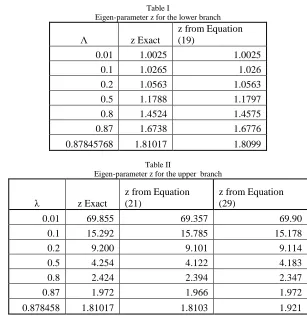
The accuracy of the approximations derived in this section is shown in table I for the lower branch and table (II) for the upper branch. Equation (19) is quite accurate for the lower branch (table I). For the upper branch one can use equation (21) for λ ≥ 0.8 and equation (29) for λ< 0.8.
Table I
Eigen-parameter z for the lower branch
Λ z Exact
z from Equation (19)
0.01 1.0025 1.0025
0.1 1.0265 1.026
0.2 1.0563 1.0563
0.5 1.1788 1.1797
0.8 1.4524 1.4575
0.87 1.6738 1.6776
0.87845768 1.81017 1.8099
Table II
Eigen-parameter z for the upper branch
λ z Exact
z from Equation (21)
z from Equation (29)
0.01 69.855 69.357 69.90
0.1 15.292 15.785 15.178
0.2 9.200 9.101 9.114
0.5 4.254 4.122 4.183
0.8 2.424 2.394 2.347
0.87 1.972 1.966 1.972
0.878458 1.81017 1.8103 1.921
It would be also of interest to find out an approximation for
2 2 2 2
1
)
5
.
0
1
log(
)
5
.
0
1
log(
1
))
log(cosh(
))
log(cosh(
1
)
0
(
)
(
x
A
x
A
A
Ax
u
x
u
(30)For large A, we will have;
x
A
Ax
A
Ax
u
x
u
1
))
log(exp(
))
log(exp(
1
))
log(cosh(
))
log(cosh(
1
)
0
(
)
(
(31)Numerical testing in the next section will show when these approximations can be used.
3. METHOD DEVELOPMENT
The Bratu problem is given by equations (1-3). Multiplying both sides by 2 du/dx and integrating with respect to x between 0 & x we obtain
0
)))
0
(
exp(
)
(exp(
2
)
(
2
u
u
dx
u
d
(32)
We now use the transformation
)
2
/
exp(
u
v
(33)To obtain
dx
dv
v
dx
du
2
(34)2 2 2 2 2 2
)
(
2
2
dx
dv
v
dx
v
d
v
dx
u
d
(35)
Substituting equations (33-34) into equation (32), we obtain;
)
1
)
0
(
1
(
)
(
2
2 2 2 2v
v
dx
dv
v
(36)Substituting equations (36) into equation (35) and then into equation (1), we obtain
0
)
0
(
2
2 2 2
v
v
dx
v
d
(37)1
)
1
(
v
(38)0
)
0
(
dx
dv
(39)Notice that from equations (33) and (4)
z
u
v
(
0
)
exp(
(
0
)
/
2
)
1
(40)So that equation (37) becomes
0
2 2 2
A
v
dx
v
d
(41)
The application of one point collocation at
x
1
1
/
5
givesthe relation
0
)
1
(
5
.
2
1 2 1
v
A
v
(42)where
v
1 is the value ofv
(
x
)
at the collocation point and thesolution is thus
)
4
.
0
1
(
2
)
1
(
1
)
(
2 2 2A
x
A
x
v
(43)The application of one point collocation at
x
1
1
/
6
givesthe relation
0
)
1
(
4
.
2
v
1
A
2v
1
(44)where
v
1 is the value ofv
(
x
)
at the collocation point and thesolution is thus
)
12
/
5
1
(
2
)
1
(
1
)
(
2 2 2A
x
A
x
v
(45))
12
/
5
1
(
2
1
)
0
(
2 2A
A
v
(46)Substituting for
A
2 from equation (14) and (40) into equation(46), we obtain the following relation for
andv
(
0
)
.1
)
0
(
5
))
0
(
1
)(
0
(
24
2
v
v
v
(47)The maximum value of
occurs at55826
.
0
)
21
1
(
1
.
0
)
0
(
v
(48)16586
.
1
))
0
(
ln(
2
)
0
(
v
Giving a value of
=0.87149 (50)We now apply a “modified collocation method” in which we collocate at x=0 in addition to the zeros of Jacobi polynomials.
For the one collocation point at
x
1=0.44721 the addition ofthe extra point at x=0 will lead to the following equations.
0
)
1
(
5
.
2
v
1
A
2v
1
(51)0
)
0
(
))
0
(
1
(
0
.
12
)
1
(
5
.
12
1
2
v
v
eA
v
e (52)We notice that the collocation equations at the zeros of Jacobi polynomials are not affected by the use of extra point.
For the present case, the solution will be correct to the second
order of
A
2 for the whole domain of x.We call the solution of the modified collocation
v
e(
x
)
12
1
4
.
0
1
24
)
2
.
0
)(
1
(
)
4
.
0
1
((
2
)
1
(
)
1
(
)
(
2 2 2 2 2 2 2 2A
A
x
x
A
A
x
A
v
x
v
e (53) and
12
1
4
.
0
1
)
60
/
1
(
)
0
(
2 2 2A
A
A
v
e (54)Substituting for
A
2 from equation (14) and solving for)
0
(
e
v
, we obtain,4 3 2 2
)
0
(
25
.
90
)
0
(
5
.
134
)
0
(
25
.
0
)
0
(
5
.
14
)
0
(
5
.
0
v
e
v
e
v
e
v
e
v
e
(55)
This gives a value of
0
.
88055
at
v
e(
0
)
0
.
55084
and
u
(
0
)
1
.
19262
Now we introduce what we call rational collocation. For multi-point collocation, one would form a rational function
)
(
x
v
r from the solutionv
(
x
)
, andv
e(
0
)
such that)
(
1
)
(
)
(
)
(
x
cP
x
cP
x
v
x
v
N N r
(56) where)
(
)
(
2 21
i N
j
N
x
x
x
P
(57)2 i
x
are the collocation points and c is a constant to beestimated such that
)
0
(
1
)
0
(
)
0
(
)
0
(
)
0
(
N N e rcP
cP
v
v
v
(58) Thus)
0
(
/
))
0
(
)
0
(
1
))
0
(
1
)(
0
(
(
N e eP
v
v
v
v
c
(59)This choice makes
v
r(
x
)
to be equal tov
e(
x
)
at thecollocation points and at
x
0
Now we apply the rational method to the one point collocation to obtain,
2
2 2
12
]
2
5
[
60
)
0
(
A
A
A
u
e
(60))
(
1
)
(
)
(
)
(
2 1 2 2 1 2x
x
c
x
x
c
x
u
x
u
r
(61)Choose c such that
2 1 2 1
1
)
0
(
)
0
(
)
0
(
cx
cx
u
u
u
r e
(62)Thus 2 1
/
))
0
(
))
0
(
1
(
))
0
(
1
)(
0
(
(
u
x
))]
1
(
4
3
)(
2
5
[(
)]
25
1
(
4
15
[
)
(
2 2
2
2 2
x
A
A
x
A
x
u
r
(65)We notice that this rational function is exact for terms up to
4
A
In addition asA
→∞,u
r(
x
)
→0 for x ε [0,1)To summarize, for λ< 0.8 on the lower branch we calculate z from equation (19), v(x) from one point collocation equation (45)and u(x) from equation (33).For λ>0.8 on the lower branch, we use equations (19,53 or 65,33) . For the upper branch, we use equations (21 or 29 ,53 or 65,33). To get better accuracy, we may go to two points or four points collocation methods. The coefficients for the second derivatives at the collocation points can be obtained from the routines in references [7-9].
4. RESULTS AND DISCUSSION
First we obtained the ratio u(x)/u(0)using the exact solution while verifying numerically the accuracy of the standard
collocation, the modified collocation and the rational
collocation methods proposed in section 3. We found that up
to
0
.
8
on the lower branch one point collocation isgood enough. We have to go to two points collocation up to the limit point and then up to 0.01 on the upper branch where we should go for four points collocation. The plots in Fig. 1 show that on the lower branch the ratio u(x)/u(0) does not change much for λ< 0.8 and approaches the parabolic profile given by equation (30). For λ< 0.01 on the upper branch the ratio approaches the straight line given by equation (31).
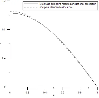
Next in Fig. 2 & 3 we show the performance of different collocation methods for λ=0.87 on the lower branch and λ= 0.01 on the upper branch. In Fig. 2, we have plotted exact solution and the numerical solution using one point standard, modified and rational collocation methods. The profiles obtained from the modified and rational collocation almost fall on the exact solution. For better accuracy we can go to two points collocation. Similarly in Fig.3 the two points modified and rational collocation almost fall on the exact solution. For better accuracy we can go to four points collocation.
Fig. 2. The lower branch u profiles for the case of
=0.87 using different collocation methods5. CONCLUSIONS
Based on a new kind of transformation, it is possible to transform the strongly nonlinear problems of Bratu equation containing an exponent term exp(u) into a linear form.
We studied the Bratu problem using different collocation methods applied to the linear form. The obtained results are found to be in good agreement with the exact solutions.
By making use of orthogonal polynomials properties, we were able to recast straightforward polynomials into a rational form. This is to be contrasted with the general procedure presented in reference [10] which could not produce a rational form as
good as the one presented in this paper.
Low order polynomials were good enough to give accurate solutions. This is in agreement with the findings of Boyd [2] that the solution is so smooth that the problem is not a strong test for numerical methods. However current research indicates that the methods introduced in this paper can prove to be very useful in treating the more challenging problem of combustion reaction in a sphere.
REFERENCES
[1] D.A. Frank-Kamenetskii, Diffusion and Heat Exchange in Chemical Kinetics, Princeton University Press, Princeton, New Jersey, 1955.
[2] J.P. Boyd, One-point pseudospectral collocation for the one dimensional Bratu equation, Appl. Math. Comp., 217: 5553-5565, 2011.
[3] H. Caglar , N. Caglar, M. Ozer, A. Valarstos, A.N.
Anagnostopoulos B-spline method for solving Bratu’s problem, Int.J. Comput. Math., 87: 1885-1891, 2010.
[4] M.I. Syam, The modified Broyden-variational method for solving nonlinear elliptic differential equations, Chaos Solitons and Fractals, 32: 392-404, 2007.
[5] A. Mohsen, On the integral solution of the one-dimensional Bratu problem”, Journal of Computational and Applied Mathematics, 251:61-66,2013
[6] C. Harley, E. Momoniat, Alternate derivation of the critical value of the Frank-Kamenetskii parameter in cylindrical geometry, J. Nonlinear Math. Phys.,15: 69–76,2008
[7] J. Villadsen and M.L. Michelsen, Solution of Differential Equation Models by Polynomial Approximation, Englewood Cliffs, New Jersey, Prentice-Hall, 1978.
[8] B.A. Finlayson, Nonlinear Analysis in Chemical Engineering, New York, McGraw-Hill, 1980.
[9] M.A. Soliman, The Method of Orthogonal Collocation, King Saud University Press, 2004. [10] J.P. Berrut, R. Baltensperger and H.D. Mittelmann, Recent