e-ISSN: 2278-7461, p-ISSN: 2319-6491
Volume 5, Issue 5 (May 2016) PP:08-28
Cost Optimization using Learning Curves and Line of Balance
Scheduling
Karim Zahran
1, Mohamed Nour
2Osama Hosny
31Comstruction Engineer & PhD student at the American University in Cairo (AUC),
2Assocaite Professor at the Architecture Department, Faculty of Fine Arts, Helwan University, Egypt,
3Professor of Civil Engineering and Construction Management, Helwan University and The American
University in Cairo, Egypt.
Abstract: Although learning curves for repetitive work have been introduced since the 1930th of the last century and despite the fact that their effect on Line of Balance (LOB) project scheduling has been under research for a long time, they have reached a plateau, where no further development of their applications have been made. This paper addresses the problem of applying cost optimization on LOB scheduling while taking into consideration the effect of learning. The paper introduces a novel approach that depends on Genetic Algorithms (GA) for optimization. Furthermore, the paper presents an application prototype that is based on a “Microsoft Excel” spreadsheet. This prototype is validated against a hypothetical case study to confirm the cost and time optimization results.
Keywords: Genetic Algorithms, Learning Curves, Line of Balance, Scheduling
I.
INTRODUCTION
After conducting an extensive literature review about learning curves and their application on Line of Balance (LOB) scheduling [1], it has been found that there is no evidence of any research work that applied cost optimization on LOB schedules while taking into consideration the effect of learning. Therefore, developing a computer model which applies the effect of both learning and cost optimization on repetitive activities, would be of great benefit to the industry. It has been found that none of the available research work exceeded the planning phase. The majority of the studies focused on the planning and scheduling phase only. Hence, there is a need for developing a tool that tracks actual learning rates, during the monitoring and control phase of a construction project, in order to continuously update the construction schedule in a dynamic manner. Table 1 summarizes the fields of focus of available research work.
After diagnosing the different techniques used for scheduling projects with repetitive activities. It was found that Critical Path Method (CPM) was introduced in the literature as having drawbacks when applied on projects with repetitive activities. It does not represent differences in production rates between activities and it requires a relatively huge number of activities to model projects with repetitive activities. Linear scheduling techniques have been introduced to overcome such drawbacks. Linear scheduling techniques have some advantages as they help planners and project managers to view the whole project in a single diagram. Moreover, they enable the user to easily get all needed information from that diagram. They easily identify relations between activities, represent the production rates for introducing the difference between productivity rates of activities, and are considered an easier way for measuring progress rates and evaluating the current performance of construction crews.
The review of current practice in scheduling repetitive projects led to the identification of some problems such as:
1. Use of the CPM by most planners and project manager for planning and scheduling repetitive projects, which has several drawbacks in scheduling such projects,
2. Ignoring the learning effect in scheduling repetitive projects
3. The unavailability of a user friendly linear scheduling tool (other than Vico control®) [2],
4. The unavailability of a linear scheduling tool which updates schedules according to actual productivity rates,
Table 1: Summery of Previous Research Work
II.
PROPOSED
COST
OPTIMIZATION
FRAMEWORK
Through the issues presented in the previous sections, an approach was developed to solve these problems. This approach is required to:
1. Apply the learning effect on LOB schedules,
2. Apply cost/time optimization to LOB schedules taking the learning effect into consideration, 3. Update learning rates, and, consequently, the LOB schedule, based on actual learning rates.
The proposed approach works according to a framework consisting of 6 modules as shown in Fig. 1. These modules are:
1. Input module
2. LOB scheduling module 3. Cost module
4. Optimization module 5. Output module
6. Monitoring and control module
On using this framework, some assumptions have to be taken into consideration, such as:
1. It is assumed that the whole project is executed continuously without any interruptions that may affect the learning rate.
2. It is assumed that quantities of all activities being executed are constant. 3. It is assumed that the learning rates are constant throughout the project duration.
4. It is assumed that same crews with similar labor and equipment are used continuously in repeating same activities. This is assumed to ensure the continuity of the learning process.
Reference LOB Scheduling Cost Optimization Learning Effect Monitoring and Control
Psarros (1987) [3]
Hegazi et al (1993) [4]
Moselhi and El Rayes (1993)
[5]
Russel and Wong (1993) [6]
Thabet and Beliveau (1994)
[7]
Lutz et al (1994) [8]
Senouci and El-din (1996) [9]
Wang & Huang (1998) [10]
Hamerlink&Rowings (1998)
[11]
Mattila& Abraham (1998) [12]
Harris &Ioannou (1998) [13]
Hegazy & Wassef (2001) [14]
Arditi et al (2001) [15]
Arditi et al (2001) [16]
Arditi et al (2002) [17]
These assumptions may not be valid in some cases; however, the model is considered self learning as it integrates previous experience from actual progress to improve the forecast for future learning rates. In addition it uses the recent learning rates for drawing the LOB schedule for future projects. This also enables it to suite several working environments according to the user inputs.
2.1. Input Module
This module is used by the user/scheduler for inputting data of the project. The user is asked to enter different types of inputs such as:
1. Project data. Information related to the project such as the project name, project code, number of repeated units, indirect cost per day, start date and target finish data (if needed).
2. Activities. Descriptions of activities and their codes for being used in later steps
3. Activity relationships. Relationships among activities and the buffer needed between them. For simplicity, this model deals with finish to start relationships only.
4. Construction method alternatives. Data about alternative construction methods for each activity (if needed). For example, the user can specify using ready mix concrete from a batch plant or mixing concrete on site for a concrete pouring activity. Each construction method is represented by its initial duration, minimum duration, direct cost/day, number of available crews and learning rate.
5. Initial Duration. The initial duration associated with each construction method specified for each activity. This is the duration the specified crew takes to finish the activity before applying the learning effect 6. Minimum duration. The least possible duration the activity can take after applying the learning effect. 7. Direct cost/day. The direct cost/day associated with each construction method specified for each activity 8. Number of available crews. The maximum available number of crews for each construction method
specified for each activity
9. The learning rate. The learning rate for each construction method specified for each activity. This learning rate can be added based on (1) previous relative databases, (2) previous experience, (3) analysis of previous related projects or (4) through updates based on actual performance on site (as shown through the monitoring and control module).
After adding all of the above parameters, these inputs are used in the calculations made in the LOB scheduling module.
2.2. LOB scheduling module
This module uses data from the input module to generate the LOB schedule of the project before and after applying the learning effect.
2.2.1. LOB scheduling without learning
Initially, the LOB schedule is calculated without the application of the learning effect. This is done through the following steps:
1. Rate of output (R) is calculated using the equation: R= Number of crews/Duration
2. The duration between the start on first unit and the start in the last unit T = (n-1) / R
where n is the number of repetitions and R is the rate of output
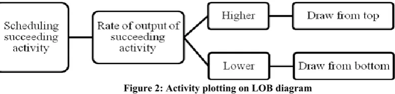
From these parameters and the assigned relationships between activities, activity bars are drawn on the LOB graph. Each bar is drawn as a parallelogram connecting the start and finish dates of the first and last units. When drawing the succeeding activity, as shown in Fig. 2, the user first has to check the rate of output of the succeeding activity. If the succeeding activity has a higher rate of output, it is scheduled from the top (starting from the last unit). If it has a lower rate of output, it is scheduled from the bottom (starting from the first unit).
Figure 2: Activity plotting on LOB diagram
As shown in Fig. 3, activity B has a lower rate of output than activity A. This means that activity B is to be drawn starting from point 1. Then the start date of activity B at the last unit is obtained by adding the “time (in days) from the start in first unit to start in last unit” of activity B and the date of point 1. For drawing the LOB bar of activity C, as shown in Fig. 3, activity C has a higher rate of output than activity B. This means that activity C is to be drawn starting from point 2 (the top). Then, the start date of activity C at the first unit is obtained by subtracting the time in days from the start in first unit to start in last unit of activity C from the date of point 2.
Finally, the LOB schedule, without applying the learning effect, is drawn and a total project duration is obtained. This schedule is calculated as a guideline for some steps in generating the LOB schedule after applying the learning effect.
2.2.2. LOB scheduling after applying the learning effect
To be able to calculate the LOB schedule while applying the learning effect, several parameters have to be calculated. The cumulative average time (CAT) is calculated using Equation 1 at each repetition, assuming that only one crew is assigned to that activity. Using the CAT, the duration of each activity at each repetition number is calculated using equation 2:
(1)
(2)
Where Durn is the duration at the repetition number n, n is the repetition number, CATn is the cumulative
average time at repetition n and is the sum of durations of all repetitions done before repetition number n. duration keeps decreasing as the number of repetitions increases until it reaches the minimum possible duration specified by the user then the duration remains constant for the remaining repetitions. Then the cumulative time is calculated using equation 3:
(3)
After calculating these parameters, the number of crews is assigned. The more crews assigned to an activity, the less the learning effect affects the durations of this activity. This happens because the number of repetitions each crew executes is fewer when having more crews. (i.e. one crew is better than two crews when considering the learning factor only).
On assigning durations for activities, the duration of executing such activity in this unit, is calculated according to the number of repetitions done by the crew executing it. This duration is extracted from durations calculated in the previous step. Later, start and finish dates of each activity at each unit is calculated.
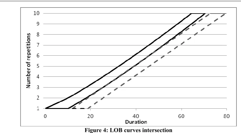
At this stage, the same concept of comparing rates of output from common LOB scheduling is applied. This means that the start date of the second activity at the first unit is taken as the finish date of the first activity at the first unit, if the rate of output of the second activity is less than the rate of output of the first activity, assuming that no buffer is defined between them. In this case, the start date of the second activity at the second unit is equal to the finish date of the first unit, assuming that only one crew is assigned. If more than one crew is applied, the number of crews is taken into consideration. This means that if two crews are assigned to an activity, then Start n = Finishn-2. On the other hand, if the rate of output of the second activity is higher than that of the first activity, then the start date of the second activity at the last unit is taken as the finish date of the last unit at the first activity, if no buffer is defined between them.
Figure 4: LOB curves intersection
Once an overlap is detected, the value of the maximum overlap between these two activities is calculated and the succeeding LOB is moved forward by this amount plus the buffer time (if assigned). After performing this check, a working LOB schedule after applying the effect of learning is generated.
2.3. Cost Module
This module is responsible for calculating the total direct cost (cost of using crews) and the total indirect cost of the project. The total direct cost is calculated by multiplying the duration of each activity at each unit by the daily cost of such crew entered by the user in the input module.
The total indirect cost of the project is calculated by multiplying the total project duration by the daily indirect cost added by the user. The model also draws the S-curve for the project through checking the working crews on a daily basis and assigning costs to these crews.
2.4. Optimization module
At this stage, the construction method applied and number of crews used are linked with the final output. This enables the user to manually adjust them to create multiples of possible combinations, of construction methods applied and numbers of crews used, which enables the user to choose an optimum LOB schedule. Assuming a project has ten activities, each activity has three different alternative methods and there are three crews available for each method. This results in 2710 (2.0589E+14) different scenarios. Hence, manual optimization of this project could take a very long time for reaching a near optimum solution. Due to the large number of possibilities, an optimization engine is needed to allow for a very large number of combinations in order to obtain a near optimum solution. To apply this optimization tool, some parameters have to be defined such as the variables, constraints and the objective function.
2.4.1. Variables
As previously mentioned, parameters such as the construction methods applied and the number of crews used for each activity are adjusted. To help reach a near optimum realistic solution, some rules have been set to reduce the amount of variables generated:
3. The construction method index has to be an integer more than or equal to one and less than or equal to the number of available alternative methods preset by the user.
4. The number of crews used has to be an integer more than or equal to one and less than or equal to the number of available crews preset by the user. It is also limited to the total number of units.
2.4.2 Constraints
Due to the type of this optimization problem, constraints are optional for the user. The user can set a total project duration for the LOB schedule or a total project cost. Once these constraints are set by the user, the program takes them into consideration during the optimization stage.
This optimization problem mainly aims at reducing the total project cost/time. The model calculates the total project cost as the sum of direct and indirect project costs. The direct cost calculated includes total daily rates of assigned crews obtained from the cost module. The total indirect cost of the project is obtained by multiplying the daily indirect cost by the total project duration. Including the indirect cost in the objective function includes the total project duration in the optimization process as well as the total project cost.
2.4.4 Optimization tool
After having variables, constraints and the objective function ready, the optimization tool is used. There are several optimization applications available (Hegazy & Wassef, 2001). One of these is Evolver which is compatible with Microsoft Excel (as a spreadsheet modeling tool). Evolver has a user-friendly interface which enables its user to link the optimization parameters to cells in the optimization spreadsheet model. Evolver utilizes genetic algorithm (GA) techniques in its calculations. GA techniques depend mainly on the idea of the survival of the fittest. It generates an initial population of different possible solutions of a problem, and only the fittest survives in the reproduction process competition. Such competition results in a near optimum solution. GA is applied in this approach as an evolutionary algorithm which has been shown to be efficient in solving such types of optimization problems with combinatorial complexity [19] (Nour et al, 2012).
In this approach, Evolver [20] works on changing the variables while taking into consideration all of the constraints, to get a near optimum total project cost/duration. While running the optimization tool, all modules are used to generate new results from the input range of suggested values for the variables. At the end of the optimization phase, a near optimum LOB Schedule is generated in a form of a table of start and finish dates of each activity at each unit.
2.5 Output module
To verify the applicability of the approach and represent its outputs graphically, a LOB graph is drawn. This LOB graph is drawn using the near optimum schedule generated from the optimization module. The LOB has an X-axis representing the unit numbers and a Y-axis representing time span (duration). LOB curved bars, due to the application of learning, are drawn by drawing two curves connecting activities’ start dates and activities’ end dates.
2.6 Monitoring and control module
After representing the LOB schedule and applying it on the project, the user is asked to record the durations at a sufficient number of repetitions at the beginning of each activity. These records are then used for monitoring the actual learning rates of each activity. This data is then used in comparing the actual durations and the preplanned durations. The difference between the actual and planned durations is calculated.
At this stage, another optimization process is needed. The optimization is run to detect the actual learning rate taking place in the project. This is done through setting the learning rate of the predicted schedule as a variable. This learning rate must have a constraint of being bigger than or equal to zero. The objective function of this optimization is to decrease the difference between the actual durations and planned durations. Once a learning rate is obtained, it is applied to the LOB Schedule.
III.
PROTOTYPE
MODEL
DEVELOPMENT
VERIFICATION
AND
VALIDATION
A computerized model is developed according to the developed framework. The model is developed using a spreadsheet modeling tool (Microsoft Excel) for scheduling the LOB and applying the learning effect. Among the advantages of spreadsheet modeling tools is their cell based structure and the user-friendly interface for non-programmers [14]. An optimization tool (Evolver Add-in on Excel) applying genetic algorithms, was used for applying cost/time optimization. Outputs of the model are presented to the user as LOB graphs. Once the user has follow-up records, related to actual production rates, such records are inserted in the model which in turn updates the LOB schedule.
3.1 Developed Prototype Model
The developed model is divided into sections similar to the division of modules presented in section II of this paper. To start a new project, the user first has to go through the input module to insert data of this project. This data is then analyzed and formulated resulting in the LOB schedule and cost reports. Finally, the user is able to use follow-up data to obtain actual learning rates and apply updated learning rates on the LOB schedule.
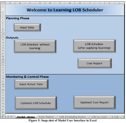
3.1.1 User interface
In order to start a new project, the user has to go through the interface in Fig. 5. This interface guides the user through the steps of using the model. First, the user has to press the “input data” button. This takes the user to the input sheet in order to add the project data. This data is then analyzed and optimized, through some working sheets, to produce the LOB schedule before and after applying the effect of learning and cost optimization. The user then has several options for choosing the contents of the output sheet. The user can press the “LOB schedule without learning” button to view the LOB schedule without applying the learning effect, or press the “LOB Schedule” button to view the LOB schedule after applying the learning effect.
The user can also chose to view the output cost report which leads to the S-curve diagram. After working with this schedule through the project, the user returns to the model interface in order to input the monitoring records. The user presses the “input monitoring data” button to be able to input data related to actual production rates on site. This data is then analyzed and formulated to produce an updated LOB schedule and cost reports. These can be viewed by pressing the “updated LOB schedule” and “updated cost report” buttons. The process of adding monitoring data about the project is considered a continuous process which can take place several times throughout the project. The following subsections show in detail steps taking place in each module in the user interface.
3.1.2 Input module
Once the user presses the “Input Data” button, the user is directed to the input module sheet shown in Fig. 6. Through this sheet, project data is inserted. Part A in Fig.6 shows the general project data which needs to be added by the user first for identifying the project. The user adds the project name, number of repeating units, the start date of the project, a target duration (if needed) and the indirect cost of the project. The user can also choose to apply cost or time optimization according to the project needs. Part B in Fig.6 shows the activity codes, descriptions, predecessors (pred.) and buffer time between activities.
Activity codes are used in the coming steps to note the activities. Part C in Fig. 6 shows data added by the user related to alternative construction methods for each activity. For simplicity, the maximum number of alternative construction methods is set to be three. The second column, in part C Fig. 6 (methods), is not a user input as it is a counter for the number of alternative construction methods each activity has. For each alternative construction method, the user has to add its initial duration, crew cost per day, learning rate of such crew and the available number of crews. Once the user finishes the input of data, he is asked to press the “Home” button to return to the user interface.
Figure 6: Input Module
3.1.3 LOB Scheduling module
Through this module, data from the input module is analyzed and formulated to produce LOB schedules before and after applying the effect of learning. It is assumed that the least total cost method is going to be applied in all activities. The number of crews is also assumed to be maximum for all activities (set as default values).
3.1.3.1 LOB Scheduling without applying the effect of learning
Part a in Fig.7 shows steps for calculating parameters needed for drawing the LOB diagram. Data as the activity code, predecessor (Pred.) and buffer are obtained from the input module. The construction method and number of crews applied are assumed to be the first method and only one crew respectively at this stage (set as default values). Later, in the optimization module, these two parameters are linked to the optimization variables to get the outputs. The duration is obtained from the input module based on the construction method applied. Based on these data, the “rate of output” and “time from start in first unit to start in last unit” are calculated.
For example, in activity B:
The “rate of output” =number of crews/duration = 4/9=0.444. The “time from start in first unit to start in the last unit” = (Number of units-1)/rate of output = (20-1)/0.444=42 days.
After calculating these parameters for all activities and considering relationships between activities, the model is able to draw the LOB schedule without applying the effect of learning.
As for activity C, it has a lower rate of output than activity B. so scheduling activity C should start from the bottom (first unit). This means that the first unit in activity C starts 5 days (buffer) after the finish of the first unit in activity B. for getting the start date of the last unit of activity C, the start of the first unit of activity C is added to the time from start of first unit to the start of last unit (Start-C20=49.6+90.3=139.9). For getting the finish dates of activity C at the first and last unit, the duration of activity C is added to these dates. The line connecting start dates and finish dates represents the start and finish dates for activity C in other units.
Based on these data, a LOB schedule (without applying the effect of learning) is drawn. Part c in Fig. 7 shows the X and Y coordinates of points used for drawing the LOB bars on Microsoft Excel. This schedule is originally based on the assumption of using maximum number of available crews and applying least total cost construction method. This schedule is drawn only for guiding later steps of scheduling and is not viewed by the model user. The LOB schedule is shown in Fig. 8. As it can be observed, the assumed data resulted in a total project duration of 202 days. This duration resulted from the application of the above assumptions without applying cost and time optimization or the effect of learning.
Figure 7: LOB schedule (without applying optimization or the effect of learning)
Figure 8: LOB Schedule after applying the learning effect
3.1.3.2 LOB scheduling after applying the effect of learning
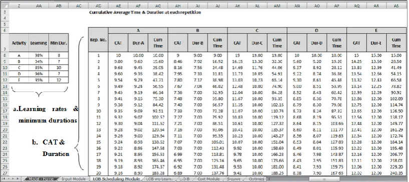
the number of units in the project, for each activity. CAT is calculated using Equation 1. Part b in Fig. 9 shows CAT and duration calculations after each number of repetitions for each activity.
For example, the CAT of activity A at repetition number four = CAT-A4 = 10x4^(log0.98/log2) = 9.6 days.
This means that the duration of activity A at the repetition number four = n x CAT – . = 4 x 9.6 – 29.05 = 9.36 days. As shown in Fig. 9, the learning effect decreases the CAT of activity A by 98% whenever the number of repetitions is doubled. This is clear in repetitions number 1, 2, 4, 8 and 16 where CAT.s are 10, 9.8, 9.6, 9.41 and 9.22 respectively. As shown in activity B duration stabilized starting from repetition number 7 at 7 days where the calculated duration became less than the minimum duration set by the user.
Figure 9: Cumulative Average Time (CAT) and duration at each repetition for each activity
A LOB schedule is then scheduled using these durations. Part a in Fig. 9 shows the calculations for generating the LOB schedule after applying the effect of learning. This schedule is prepared based on the use of only one crew, so durations at each unit number is similar to the duration at that number of repetitions calculated in part b in Fig. 9. As for activity A, units are scheduled back to back where a construction crew finishes the first unit then starts in the second unit and so on. This completes up to the last unit. To schedule activity B, the relation between rates of activity A and B, before applying learning, must be checked first. Same concept of scheduling based on difference in rates, applied in common LOB scheduling, is applied in this case. Based on the case study, the rate of output of activity B is higher than activity A. so scheduling activity B starts from the last unit. So :
Start-B20 = Finish-A20 + 5 (buffer).
This means that activity B has to be scheduled backwards, where: Start-Bn= Finish-Bn+1.
Same concept applies to activity C, where the rate of output of activity C is lower than activity B. This means that scheduling activity C starts from the first unit. So:
Start-C1 = Finish-B1 + 5(buffer)
And later units come next according to the finish dates of crews at each unit. So: Start-Cn = Finish-Cn-1, and this completes to the end of the activity.
Figure 10: LOB Schedule (after applying the learning effect) and overlap check
In this case study, an overlap took place between activity C and activity D after applying the learning effect. This is shown in part b of Fig. 10. This part detects the units having an overlap between each two activities. Once an overlap is detected, part c in Fig.11 calculates the value of the overlap at each unit between these two activities. Highlighted cells in each column are the maximum values of overlap. The maximum amount of this overlap is calculated at the top of part c. Then, the succeeding activity is moved forward by the value of the overlap (taking into account buffer if it exists). In this case, an overlap was detected between activities C and D. The value of this overlap was calculated to be 2 days. So activity D had to be moved forward by 2 days to result in the new start and finish dates of activity D in part a of Fig.11. In this case, after activity D was moved forward, the overlap check between activity D and activity E had to be done for activity D after being moved forward (in part of Fig.11). This showed that the overlap between activity D and activity E took place after moving activity D forward by 2 days, which resulted in moving activity E 2 days too. As shown in the overlap between activity C and D, the maximum overlap took place between these two activities in unit number three, as previously explained in Fig.4.
The generated LOB schedule, at this stage, is not presented to the user as it is based on assumptions of using maximum number of crews and applying the least total cost construction method.
This schedule is generated on an automated spreadsheet model to facilitate the optimization process in later steps. As shown from the case study, the total project duration decreased to 173 days after applying the effect of learning. This means that the learning effect, decreased the total duration of the project by 28 days (14%).
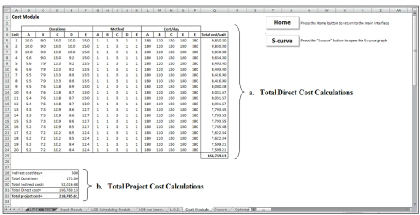
Figure 12: Cost Module
3.1.4 Cost Module
In this module, cost data provided by the user in the input module is used to generate total cost of the project. This module is concerned with crew costs and in-direct costs only. It is assumed that whatever effects learning has on activity durations, it does not affect costs of materials used in construction. Part a in Fig. 12 shows calculations made for getting total direct cost of the project. It has the durations of each activity at each unit, construction method applied, and cost per day associated with these construction methods. Based on these data, a total cost per unit is calculated which is the sum product of durations of activities and their cost per day for that unit. From these total costs per unit, a total direct cost for the project is calculated by summing them up.
Figure 13: S-Curve Calculations
The indirect cost of the project is calculated by multiplying the total project duration by the indirect cost per day of the project. The total project cost is obtained by adding the total indirect cost and total direct cost.
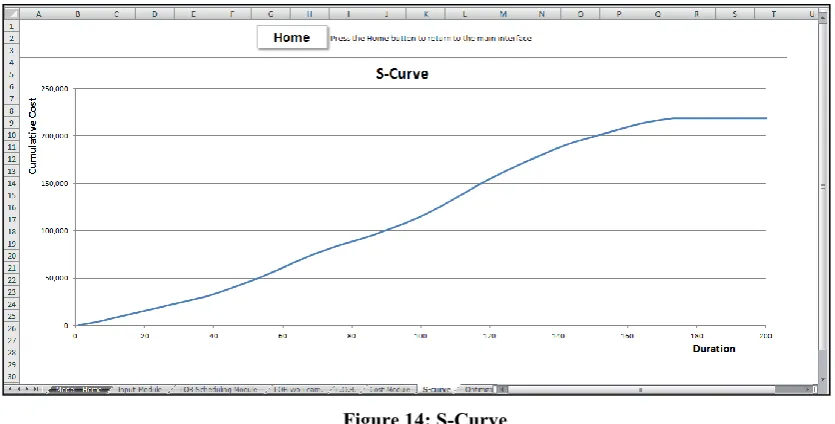
summing the costs of all preceding days. The S-curve drawn is shown in Fig. 14 as the plot of the cumulative cost over time.
Total cost of the project in the case study, on using maximum number of crews, applying the learning effect and applying the minimum total cost construction method, was218,785. This cost and the S-curve were not viewed by the user as they were formulated in preparation for the next step of applying optimization to the LOB schedule.
Figure 14: S-Curve
3.1.5 Optimization module
The optimization module is responsible for applying cost and time optimization to the LOB schedule. Part a in Fig. 15 shows the model setting for applying the optimization engine. First activities are identified. The highlighted columns represent the model variables. These are the construction method (numbering) and the number of crews used. Based on the construction method chosen, the duration, cost per day and learning rate are extracted from the input module.
Part b in Fig. 15 shows the setting of constraints for use in the optimization process while changing variables. These constraints are set based on the inputs of the user. As for activity A, the user set three different construction methods. This means that changing the construction method must be an integer bigger than or equal to one and smaller than or equal to three. Based on the chosen construction methods, the limits for the number of crews used are set. In activity A, the user set a maximum of three crews in the first method. So the number of crews chosen has to be an integer bigger than or equal to one and smaller than or equal to three. This data is then processed through the previous modules to get the total project duration and total project cost.
Fig. 16 shows the user interface of Evolver add-in on Microsoft Excel. Section 1 shows the optimization goal set to minimize the total project cost; the user can also set the optimization goal to minimize the total project duration if cost is not of concern. Section 2 shows the identification of the project variables and the limitations on changing these variables. Section 3 shows the constraints on the output optimization process. Once these parameters are set, the model is ready to run. After running the model, a near optimum combination of model variables is generated.
Figure 16: Evolver Optimization Settings
Part a in Fig. 17 shows the results of the optimization process on the case study. The optimization process resulted in a total project cost of 215,770 instead of the initial project settings which resulted in a total project cost of 218,786. Also the total project duration decreased from an initial duration of 344 days to 253 days.
3.1.6 Output Module
Figure 18: LOB Schedule after applying optimization and the effect of learning
Figure 19: S-curve (after optimization)
Fig. 18 shows the resulting LOB schedule after applying cost optimization and the effect of learning. The user views this LOB schedule on pressing the “LOB schedule” button in the user interface shown in Fig. 5. Straight curves represent the start dates of each activity while dashed curves represent finish dates.
Figure 19 shows the S-curve generated after applying the effect of learning and cost optimization. The user can view this figure by pressing the “Cost Report” button in the user interface in Fig. 5.
After the user applies the LOB schedule generated from the previous module, duration records from site are used for adjusting the LOB schedule. This stage is useful in adjusting the initial durations and learning rates according to the working environment. At this stage, the user has to press the “Input actual data” button in the user interface in Fig.5 . Once the user presses that button, he is directed to the monitoring data input sheet.
Fig. 20 shows data, the user has to add to the model. It also shows the assumed data for using this module related to the case study. The user has to add durations for a specific activity at each unit number for a reasonable number of repetitions.
Figure 21: Monitoring and Control Module (before getting actual learning rates)
Data added by the user is then added in Figure to get the actual learning rate on site. The first three columns show actual data added by the user. The second three columns show CAT and durations calculated based on the learning rate used in the LOB schedule. The error column at the right represents the difference between actual durations and planned durations. An optimization process is needed to try matching the planned and actual
durations. This is done by applying an optimization tool for decreasing the total value of errors. This problem is considered a simple optimization, so it could be done using Solver add-in on Microsoft Excel.
Figure 22: Solver Settings
Fig. 22 shows settings for the solver add-in to apply the optimization problem. As shown in the figure the total error is set be minimized while the learning rate cell is set to be the variable. Once this optimization process is finished, an actual learning rate is generated (as shown in Fig. 23).
Whenever the user adds actual durations, the model calculates learning rates and uses them in adjusting the LOB schedule and costs. Actual learning rates are inserted in the LOB scheduling module to generate the updated LOB schedule which is then used by the cost module to generate the updated cost report. These are viewed by the user by pressing the “updated LOB schedule” and “Updated Cost report” buttons in the user interface.
IV.
RESULTS
AND
DISCUSSIONS
After applying the model to the hypothetical case study, an analysis of the results was done. Results of the model were divided into three categories: (1) using common practice of LOB scheduling, (2) after applying the learning effect, and (3) after applying both the learning effect and cost optimization. The comparison was done on three bases:
1. Total project duration 2. Total project cost 3. S-curve
4.1 Total project cost comparison
Figure shows a comparison between the total project cost of the three categories:(1) original LOB, (2) LOB after applying the learning effect and (3) LOB after applying cost optimization. As shown in the figure, the total project cost decreased by 14% after applying the effect of learning. It also decreased by another 12% after applying cost optimization. This means a total of 26% savings in the total project cost.
Figure 24: Total project cost comparison for hypothetical case study
4.2 Total project duration comparison
Figure 5 shows a comparison between the total project duration of the three categories: (1) original LOB, (2) LOB after applying the learning effect and (3) LOB after applying cost optimization. As shown in the figure, the total project duration decreased by 12% after applying the effect of learning. It also decreased by another 1% after applying cost optimization. This means a total of 13% savings in the total project duration. The effect of the optimization process on the total duration was not as significant as it was on the total project cost, as the optimization process was set to optimize total project cost.
4.3 S-curve comparison
Figure shows a comparison between the s-curves of the three categories, original LOB, LOB after applying the learning effect and LOB after applying cost optimization. As shown in the figure, the S-curve of the optimized LOB (dashed curve) had higher cumulative values at the beginning of the project until it reaches a cumulative cost of 215,770 at a total project duration of 148 days. However, the S-curves of the original LOB (straight curve) and the LOB after applying the learning effect (dotted curve) kept intersecting at the beginning of the project, then the S-curve of the LOB after applying the learning effect became higher when approaching the end of the project. This can be caused by the learning effect where it has a higher effect as the number of repetitions increases (nearer to the end of the project).
Figure 26: S-curve comparison for hypothetical case study
V.
CONCLUSIONS
AND
RECOMMENDATIONS
FOR
FURTHER
RESEARCH
This paper introduced steps of developing the model based on the proposed methodology. These steps were shown on a hypothetical case study at first to show all of the model capabilities. These steps started from introducing the interface the user has to use to start a new project. Then through the input module the user enters data about the project. These data are then formulated through the LOB scheduling module to obtain the LOB schedules before and after applying the learning effect. This LOB schedule is then used along with cost data added by the used in the cost module to produce cost reports and draw the S-curve. Then the optimization module is responsible for reducing the total project cost through changing construction methods and numbers of crews used. This results in an optimized LOB schedule which is then viewed by the user through the output module. Finally, after the user applies the LOB schedule in site, monitoring data is then used to continuously adjust the durations and learning rates according to actual rates.
In addition, this research presented a prototype model for proving the validity of the proposed approach. This model was developed using a spreadsheet modeling tool for scheduling the LOB and applying the learning effect. Moreover, an optimization engine, applying genetic algorithms, was used for applying cost/time optimization on the same model.
The presented prototype model was verified by applying it on a hypothetical case study. This application verified that rules applied were appropriate and that the model gives accurate results. Moreover, a comparison between common LOB scheduling, application of learning effect and the application of cost optimization was done. This comparison introduced the ability of the proposed model to decrease the total project cost, total project duration and improve the efficiency of usage of resources.
This study presented a framework capable of assisting planners/schedulers in including the learning effect and cost/time optimization in scheduling projects with repetitive nature. A model was designed to apply the presented framework. However, in order to enhance its capabilities, the following recommendations can be considered in future research:
An add-in to any of the scheduling tools, applying the proposed model, could be generated to facilitate the application of the proposed approach
Adding non-linear activities to the scheduling process
The current model only accepts finish to start relationships between activities; however, it could be extended to accept other relationships between activities
Add a resource constraint for limiting the maximum number of resources which can be used in a specific duration. This can be considered for activities which share the same resources
Include interruptions as a variable in the optimization process while taking into consideration the effect of learning and forgetting curves
Include a dynamic change of the number of crews according to the learning forecast and actual performance. i.e. to decide when to drop off extra crews or when to implement extra crews towards the end of the project
Include other alternatives such as using night/day shifts or overtime for same crews taking into consideration the decrease in productivity and time/cost tradeoff
REFERENCES
[1] Zahran k., Nour M. and Hosny O. The Effect of Learning on Line of Balance Scheduling: Obstacles and Potentials, International Journal of Engineering Science and Computing, IJESC, Volume 6 Issue No.4 April 2016, under publication.
[2] Vico Software, VICO control Classic. 2016 http://www.vicosoftware.com/products/Vico-Control/tabid/84573/ , last accessed 13th of March 2016.
[3] Psarros, M. E. SYRUS: A Program for Repetitive Projects. Master's Thesis, Department of Civil Engineering, 1987, Illinois Institute of Technology, Chicago, IL.
[4] Hegazy, T., Moselhi, O., & Fazio, P. BAL: an agorithm for scheduling and control of linear projects. 1993. AACE Transactions, 8.1-8.14
[5] Moselhi, O., & El-Rayes, K. Scheduling of repetitive projects with cost optimization. Journal of Construction Engineering and Management , 1993. 199(4), 681-697.
[6] Russel, A. D., & Wong, W. C. New generation of planning structures. Journal of Construction Engineering and Management, 1993. 119(2), 196-214.
[7] Thabet, W. Y., & Beliveau, Y. J. HVLS: horizontal and vertical logic scheduling for multistory projects. Journal of Construction Engineering and Management, 1994. 120(4), 875-258.
[8] Lutz, J. D., Halpin, D. W., & Wilson, J. R. Simulation of learning development in repetitive construction. 1994, Journal of Construction Engineering and Management, 120(4), 753-773.
[9] Senouci, A. B., & Eldin, N. N. Dynamic programming approach to scheduling of non serial linear projects. Journal of Computing in Civil Engineering, 1996, 10(2), 106-114.
[10] Wang, C., & Huang, Y. Conrolling activity interval times in LOB scheduling.Construction Management and Economics, 1998, 16, 5-16.
[11] Hamerlink, D. J., & Rowings, J. E. Linear Scheduling Model: development of controlling activity path. Journal of Construction Engineering and Management, 1998, 124(4), 263-268.
[12] Mattila, K. G., & Abraham, D. M. Resource leveling of linear schedules using integer linear programming. Journal of Construction Engineering and Management, 1998, 124(3), 232-244.
[13] Harris, R. B., & Ioannou, P. G. Scheduling projects with repeating activities. Journal of Construction Engineering and Management, 1998, 124(4), 269-278.
[14] Hegazy, T., & Wassef, N. Cost Optimization in Projects with Repetitive Nonserial Activities. Journal of Construction Engineering and Management, 2001, 127(3), 183-191.
[15] Arditi, D., Tokdemir O. B., & Suh, K., Effect of learning on line of balance scheduling. International Journal of Project Management, 2001, 19 (5), pp. 265-277.
[16] Arditi, D., Tokdemir O. B., & Suh, K., Scheduling System for repetitive unit construction using line of balance technology. Journal of Engineering Construction and Architectural Management, 2001, 8 (2), pp. 90-103.
[17] Arditi, D., Sikangwan, P., & Tokdemir, O. B. Scheduling system for high rise building construction. Construction Management and Economics, 2002, 20(4), 353-364.
[18] Tokdemir, O. B., Arditi, D., & Balcik. ALISS: Advanced Linear Scheduling System. 2006, Construction Management and Economics, 24(12), 1253-1267.
[19] Nour, M., Hosny, O., & Elhakeem, A. A BIM based Energy and Lifecycle Cost Analysis/Optimization Approach. International Journal of Engineering Research Applications, 2012, 2(6), 411-418.