Paper 11-2017-1

(1)

(DOI: 10.24874/jsscm.2017.11.01.11)

Eigenvalues and Three-Term Approximation of Fourier Series Solution of

Heat Conduction Transients, Valid for 0.02<Fo<

∞

and All Bi

A. Ostrogorsky1

1 _{Illinois Institute of Technology} e-mail: [email protected]

Abstract

For transient conduction/diffusion driven by convection boundary conditions, in plates, cylinders and spheres, a set of correlations is presented providing explicit one-, two- and three-term approximations of Fourier series solution. The correlations yield eigenvalues (λ1, λ2 and λ3)

and coefficients (A1 ,A2 and A3) with less than 0.6 % error. The correlations are more precise

than tables or charts available in textbooks, and do not require interpolation between given values or curves.

Keywords: Eigenvalues, heat conduction, diffusion, Fourier series.

1. Introduction

Transient heat conduction problems in finite solids with convective boundary conditions are common. While exact analytical solutions are available, their precision is limited by the ± 10 % uncertainty in the convection heat transfer coefficient h and Biot number,

hL Bi

k

=

where k is thermal conductivity and L is characteristic length.

Frequently, finite solids can be approximated as plates, cylinders and spheres. Thus, analytical solutions of heat conduction transients remain useful for engineering calculations and education. Early “surface” transients driven by convection are modeled using the semi-infinite solid solution along the surface assumed to be flat (Glicksman and Lienhard 2016, Lienhard and Lienhard 2017, Incropera and De Witt 1990, Kakac and Yener 1993, Arpaci 1966):

( )

, ₂ 2

( )

x t

erf e erfc

i

θ _{βη β}

η η β

θ = + + + (1)

1

2 2

x

t Fo

ξ η

α

(2)

h t

Bi Fo k

α

β = =

where x1=L-x is distance from the surface. Fourier number is defined as:

2 t Fo L α =

where t is time, α is thermal diffusivity. L is ½ plate thickness. For cylinders and spheres, L is replaced by R.

Fourier series solution for finite solids can be presented in the following concise form (Glicksman and Lienhard 2016):

2 n 1 f Fo n n n

i f i

T T

A f e

T T λ θ θ ∞ − = − = =

−

∑

(2)

Coefficients An, functions fnand eigenvalue equations for λn are given in Table 1. where

ξ=x/L or ξ=r/R.

Fourier series in Eq. (2) converges rapidly, because of the negative argument of the exponential term, _e−λn Fo2 _{. One term is sufficient for}_Fo>_{0.2 (Glicksman and Lienhard 2016,} Lienhard and Lienhard 2017). The key obstacle preventing frequent practical use of Eq. (2), are eigenvalue equations, which are transcendental. λn appears two times in each equation, which

has to be solved numerically. For practical engineering calculations, most textbooks provide: i. Tabulated values of λ1 and A1 (Glicksman and Lienhard 2016, Incropera and De Witt.

1990). Carslaw and Jaeger (1959) provide the first six eigenvalues.

ii. Transient response charts, e.g. Heisler charts (Heisler 1947) for 0.2<Fo<700 [3,4] or charts for the range 0<Fo<1.5 (Lienhard and Lienhard 2017, Arpaci 1966).

Schneider’s monograph (Schneider 1963) contains numerous high-resolution charts, extending the range of Fourier numbers to Fo =0.001. More recently (Ostrogorsky 2009), we provided a set of correlations for λ1 and A1 as a function of Bi. These are applicable for Fo>0.2

and all Bi, with<1 % error (Glicksman and Lienhard. 2016, Ostrogorsky 2009).

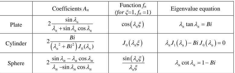
Table 1. Coefficients, functions and eigenvalue equations for Eq. (2) (Glicksman and Lienhard 2016, Lienhard and Lienhard 2017)

Coefficients An Function fn

(for ξ=1, fn =1)

Eigenvalue equation

Plate n

n n n

sin 2

sin cos λ

λ + λ λ cos

( )

λ ξ

n λntanλ =n Bi

Cylinder

(

2 2

)

n 0 n

2

( )

Bi Bi J

λ + λ J0

( )

λ ξ

n

λ

nJ1

( )

λ

n −Bi J0

( )

λ

n =0

Sphere 2 sin cos sin cos

n n n

λ λ λ

−

( )

_n n

sin λ ξ

(3)

2. Correlations for eigenvalues and coefficients

Our goal is to present a set of explicit three-term approximations of the Fourier series solution, that can be used for all Biot numbers in the time-range not covered by Eq. (1). For plates, cylinders and spheres these approximations are:

(

)

2

1 cos n m Fo n n n i plate

A e λ

θ _{λ ξ}

θ

−

=

∑

(3)

( )

2

0 1 n m Fo n n n i cyl

A J e λ

θ _{λ ξ}

θ

−

=

∑

(4)

(

)

2

1 sin n m Fo n n n

isph n

A λ ξ e λ

θ

θ = λ ξ −

=

∑

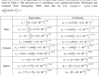
(5)

where m=1, 2 or 3. The eigenvalues λ1, λ2, and λ3 and Fourier’s coefficients, A1, A2 and A3 are

listed in Table 2. The one-term (m=1) correlations were reported previously (Glicksman and Lienhard 2016, Ostrogorsky 2009). Note that for ξ=0, cos 0

( )

=1, J₀

( )

0 =1and

( )

0

lim sin 0 / 0 1

x→  = .

Table 2. Explicate correlations for eigenvalues and coefficients

3. Exact solutions and correlations

Eigenvalues Coefficient

Plate

(

)

0.468

1.07 1 1 2.62 /

2 Bi

π

λ

= + −

(

_1.5

)

2/3

1 1 0.273 1 2.42 /

A = + + Bi −

(

)

0.833

1.2

2 1 6.733 /

2 Bi

π

λ = +π + − _1.45 1/1.45

2 0.4244 1 3.5 /

A = − _ + Bi _−

(

)

0.9

1.11

3 2 1 10.5 /

2 Bi

π

λ = π + + − _1.63 1/1.63

3 0.2546 1 15.3 /

A = _ + Bi _−

Cylinder

1.7

)

0.588

3 0.85 1 24 /

A = + Bi −

)

0.833

1.2 3 7.72 1.7 1 16 /Bi

λ

= + + −

(

1.8

)

0.556

3 2 1 40 /

(4)

exact with five significant digits. lamda_1, lamda_2 and lamda_3 are calculated using the correlations given in Table 2.The correlation error:

[ ] _

% 100

[ ]

num n lamda n error

num n

−

= × (6)

is below 0.6 %, see Figs. 1b, 2b and 3b.

Fig. 1. a) num[1], num[2] and [3] are numerical solutions of the eigenvalue equation for plates, Table 1. lamda_1, lamda_2 and lamda_3 were calculated using correlations in Table 2; b) Error

< 0.43 %

Fig. 2. a) num[1], num[2] and [3] are numerical solutions of the eigenvalue equation for

(5)

Fig. 3. a) num[1], num[2] and [3] are numerical solutions of the eigenvalue equation for

spheres, Table 1. lamda_1, lamda_2 and lamda_3 are correlations given in Table 2. b) Error < 0.6 %

In Figs. 4 to 8, Eqs. (3), (4) and (5) with m=1 to 3, are compared to the exact solutions (10-term Fourier series, full lines labeled Exact). Dashed blue line with circles represent the semi-infinite solid model, Eq. (1). Errors in dimensionless temperature are:

.

% exact approx 100

i

error θ θ

θ −

= × (7)

Plates having 2L thickness “behave” as semi-infinite, as long as the transient penetration depth δ is less than L. Thepenetration depth is:

3.65 t 3.65L Fo

δ

=

α

= (8)

settingδ= L in Eq. (8) gives Fo=0.075. Therefore, the semi-infinite solid solution is expected to

be virtually exact for 0<Fo≤0.075. Accordingly, for Fo=0.075 and Bi=10, Eq. (1) gives <0.55%

(6)

The semi-infinite solid model can be applied to cylinders and spheres for a short period of time, while transient penetration depth δ is small compared to R (δ <<R), InFig. 5a, Fo=0.055 was chosen because at that time δ = R1_{. For}δ₌_R,_{Eq. (4) with three terms (}_m_{=2) is}

exceptionally precise, giving <0.25 % error. However, the semi-infinite solid model requires δ

<<R and thus yields 6.49 % error, see Fig. 5b.

Fig. 5. Cylinder, Fo=0.055, Bi=10. a) Dimesionless temperature profile; b) % error. SI is Eq. (1) T1+T2 and T1+T2+T3 are Eq. (4) with m=2 and m=3 respectively

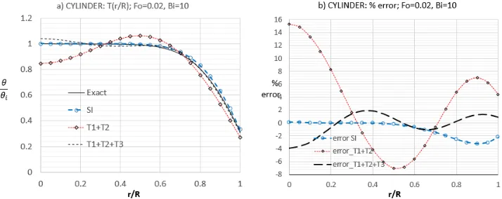
In Fig. 6a, δ ≈ ½ R correspondstoFourier number Fo=0.02. As a result, error in Eq. (1) is reduced to<3.22 %, while Eq. (4) with three-terms (T1+T2+T3), gives < 3.9 % error, Fig. 6b.

Fig. 6. Cylinder, Fo=0.02, Bi=10. a) Dimesionless temperature profile; b) % error. SI is Eq. (1) T1+T2 and T1+T2+T3 are Eq. (4) with m=2 and m=3 respectively

(7)

Fig. 7. Sphere, Fo=0.045, Bi=10. a) Dimesionless temperature profile; b) % error in SI model, Eq. (1). T1+T2 and T1+T2+T3 are Eq. (5) with m=2 and m=3 respectively

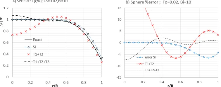
In Fig. 8. to make the precision of Eqs. (1) and (5) more even, Fourier number is set to Fo=0.02. As a result, Eq. (1) gives <6.5% error while Eq. (5) with three-terms (T1+T2+T3,

m=3), gives 7.4 % error at r/R=1. Error is <2 % for 0.25<r/R<1 (see Fig. 8b).

Fig. 8. Sphere, Fo=0.02, Bi=10. a) Dimesionless temperature profile; b) % error. SI is Eq.(1)

4. Conclusions

(8)

see Table 2. The correlations yield: <0.42 % error for plates, <0.5 % for cylinders and <0.6 % for spheres (see Figs. 1-3).

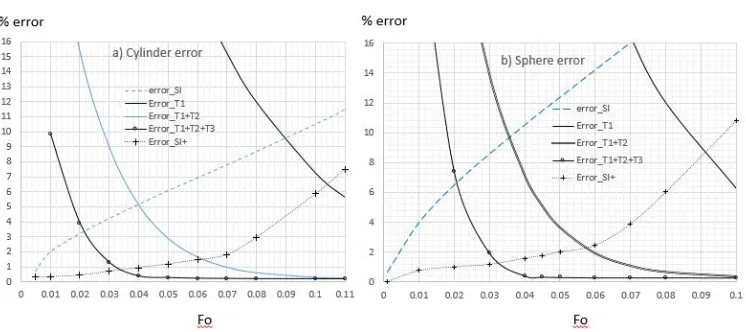
Figure 9 shows the errors in the semi-infinite solid solution, Eq. (1) and proposed Eqs. (4) and (5). Considering the +/- 10 % typical uncertainty in Biot numbers, <2 % error appears appropriate for practical calculations. Therefore, the useful time-range of the semi-infinite solid solution should not be starched beyond Fo≈0.005 for cylinders and Fo≈0.01 for spheres. In conclusion, based on the errors shown in Fig. 9, the following is recommended:

• Semi-infinite solid solution, Eq. (1), should be used in the range 0<Fo<0.01 for cylinders and 0<Fo<0.005 for spheres.

• Two-term approximation should be used in the range 0.06<Fo<∞; • Three-term approximation should be used in the range 0.03<Fo<∞.

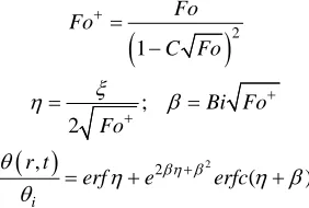
Note: The recently proposed “extended” semi-infinite solid model (Ostrogorski and Mikic, 2017), dotted line with + in Fig. 9 is sufficiently precise in the 0< Fo ≤ 0.06 range. This “extended” semi-infinite solid solution combines Eq. (1) with effective or “extended” Fourier number, Fo+_:

(

)

( )

2

1 ; 2 ,

( )

i

Fo Fo

C Fo

Bi Fo Fo

r t

erf e βη β erfc

ξ

η β

θ

η η β

θ

+

+ +

+

= −

= =

= + +

(9)

where C=½ for cylinders and C=1 for spheres. Fo is standard Fourier number based on radius R,

2 t Fo

R

α =

(9)

Fig. 9. Error in semi-infinite solid (SI) solution, Eq. (1) and a) Eq. (4) for cylinders and b) Eq. (5) for spheres. T1, T1+T2, and T1+T2+T3 correspond to one- two- and three-term approximations. Error SI+_{is error in Eq. (9) with a)}_C_{=½ for cylinders, and b)}_C_{=1 for spheres}

Acknowledgment The author would like to thank Professor John Lienhard of Massachusetts Institute of Technology, for valuable suggestions and interest in this project.

References

Arpaci V (1966). Conduction Heat Transfer, Addison-Wesley, Reading, MA.

Carslaw and Jaeger (1959). Conduction of Heat in Solids, Oxford Univ. Press, 2nd ed.

Glicksman LR, and Lienhard VJH (2016). Modeling and Approximation in Heat Transfer, Cambridge University Press.

Heisler MP (1947). Temperature Charts for Induction and Constant-Temperature Heating, Trans. ASME, 69, 227–236.

Incropera FP and De Witt DP (1990). Introduction to Heat Transfer, 2nd ed., Willey, New York.

Lienhard JH IV and Lienhard JH (2017). A Heat Transfer Textbook, 4th ed. Phlogiston Press, Cambridge MA. http://ahtt.mit.edu

Kakac S and Yener Y (1993). Heat Conduction, 3rd ed., Taylor & Fancis, London.

Ostrogorsky AG (2009). Simple Explicit Equations for Transient Heat Conduction in Finite Solids, ASME J. Heat Transfer 131 011303-1.

Ostrogorsky AG and Mikic BB (2017). Semi-infinite solid solution extended to cylindrical and spherical solids, using time dependent participating volume-to-surface ratio and erfc solutions”, ASME J. Heat Transfer, submitted.