Forestry & Natural-Resource Sciences Last Correction: Feb. 16, 2010
COMPARISONS OF THREE DIFFERENT METHODS USED TO
GENERATE FOREST LANDSCAPES FOR SPATIAL HARVEST
SCHEDULING PROBLEMS WITH ADJACENCY RESTRICTIONS
Rongxia Li
1, Pete Bettinger
2, Aaron Weiskittel
31Postdoc,3Assistant Professor, SFR, University of Maine, Orono, ME 04473 USA 2Professor, WSFNR, University of Georgia, Athens, GA 30602 USA
Abstract. Dealing with adjacency constraints is currently one of the main research focuses of spatial
harvest scheduling problems. In many situations, hypothetical landscapes are generated for research purposes. The simulation methods used to produce hypothetical landscapes are important and may affect the planning solutions. In this study, we examined three landscape simulation methods (grids, Voronoi diagrams, and random graphs) and compared them to a forest developed using irregularly-shaped polygons within a geographic information system. The effects on the optimal planning solutions due to different spatial layouts were investigated as well. The results show that landscape simulation methods have a significant impact on the mean solution values and CPU running time due to different adjacency patterns in each simulated landscape. Advantages and disadvantages using each of the three methods are discussed and useful suggestions are provided regarding the selection of one particular method for research purposes.
Keywords:Simulation, Voronoi diagrams, random graphs, grids, adjacency constraints
1
Introduction
The spatial layout of forestry operations can have a profound impact on many non-timber objectives (T´oth and McDill, 2009). In accordance with the increasing concerns of ecological and social functions, such as recre-ational use, forest aesthetics, and wildlife habitat, and in conjunction with timber supply goals, spatial forest planning has been introduced into the forestry practice and has become increasingly important over the past two decades (Bettinger and Sessions, 2003). To accom-modate the requirements of forest policies and concerns from different aspects, forest managers and researchers attempt to address forest planning issues in a spatially explicit context.
Since it is often logistically difficult, time consum-ing, and cost-prohibitive to obtain the real world for-est landscape data, hypothetical forfor-est landscape data have largely been used in many spatial forest planning research studies. Using hypothetical forest landscape data is not just a second option when the available real world data are limited. In fact, it is preferred in many situations because hypothetical landscapes can be re-peatedly generated, thus it is possible to control certain factors at a predefined level and perform various
hy-pothesis tests on the final planning solutions. Compared with real-world applications, the confounding effects due to white noise (i.e., non-important or un-identified fac-tors) can be easily removed or minimized in a hypothet-ical dataset. For example, to examine whether spatial patterns of landscapes have an impact on planning solu-tions, a typical forest planning problem can be solved for various hypothetical landscapes which differ only in the spatial pattern of management units (e.g., clustered, dis-persed), while maintaining the same attributes of those management units (e.g., growth rates of forests, size of management units).
The most common way to generate a hypothetical landscape is to generate grids or mosaics, where each cell represents a forest stand (e.g., Barrett et al., 1997; Van Deusen, 2001; Bettinger et al., 1997; Chen and van Gadow, 2002). However, due to the regularity of grids, this method has many limitations which may pre-vent us from finding further embedded problems. Other landscape simulation methods have also been proposed in the forestry literature, such as the Voronoi diagram (e.g., Kurz et al., 2000; Thompson et al., 2009) and random graph methods (e.g., Crowe et al., 2003; Gunn and Richards, 2005). Although most research studies in this latter case do not explicitly mention the random
graph method, many involve randomly developed graphs drawn by hand as illustrations, and the concept behind those graphs are consistent. McDill and Braze (2000) also developed a Visual Basic program (MAKELAND) to generate random hypothetical landscapes. Each simu-lation method results in landscapes with different spatial layouts. How the spatial layout affects the research anal-ysis and conclusions, and the impact on plans remains unknown.
Today, one of the key elements in a spatial forest plan-ning problem is the adjacency constraints. When using these constraints, the prescribed treatments on neigh-boring stands have a restrictive impact on the decision of current stand treatments. It has been widely acknowl-edged that adjacency constraints are critical and greatly affect forest planning solutions. A number of research studies describe how adjacency constraints can be in-corporated into forest plans. For example, Murray and Church (1995) examined various structural representa-tions of adjacency condirepresenta-tions in forest planning prob-lems. Zhu and Bettinger (2008) studied the impact im-posed by different spatial land patterns (random, clus-tered and dispersed) on harvesting plans for loblolly pine stands in the southern United States. And Nalle et al. (2005) studied the economic impact caused by first and second order adjacency constraints and green-up straints in the western United States. First-order con-straints limit harvesting opportunities in physically ad-jacent stands, while second-order constraints do this as well as limit harvesting opportunities in stands that bor-der a stand scheduled for harvest. However, we rarely find studies that aim to investigate how different adja-cency structures affect solutions of the spatial harvest planning. For example, a landscape with an average of four adjacent neighbors may behave differently from a landscape with an average of eight neighboring stands in a spatial forest planning context. The influence of these vertex degrees (the average number of stands that are adjacent to a given stand in the forest) are of interest to this study.
In sum, the objectives of this study were 1) to gen-erate forest landscapes using grids, Voronoi diagrams, and random graph methods; 2) to apply a typical spa-tial forest planning problem to landscapes generated by the these three methods; and 3) to compare the optimal solutions and examine how spatial layout and adjacency constraints affect the planning solution values. The dis-cussion will be centered on the advantages and disadvan-tages of using different simulation methods, and we hope that forest researchers can benefit from being aware of pros and cons of using each of the above three methods in simulating the hypothetical forest landscapes for their research purposes.
2
Methods
This section begins with the description of the forest data used for comparing the different approaches, fol-lowed by a description of the three different approaches for developing spatial relationships among the forested stands. At the end of this section, a description of the forest planning problem to be solved is presented.
2.1 Forest Landscape Data We used the Daniel Pickett Forest from the bookForest Management (Davis et al., 2001) as our example data. Originally, the database included 73 stands, and we extracted 49 stands for our current study due to the computational restric-tions of the student version of CPLEX. Each stand is associated with a unique identification number and two non-spatial attributes: stand area size (acres) and tim-ber volume (MBF, or thousand board feet per acre) it is capable of producing in each of three time periods (decades). All of the stands either increase in volume over time or (when they are very old) the volume re-mains constant. In addition, all of the stands are eligible for harvest in each time period.
2.2 Simulating Landscapes using Three Differ-ent Methods In order to perform a statistical analysis on the planning solutions using three different simulation methods (grids, Voronoi diagrams, and random graphs), we created 30 landscapes using each method with cer-tain specifications. For each landscape, 49 stands were simulated, and stand identification numbers and the cor-responding stand attributes (timber volume production and stand area) obtained from the Daniel Pickett Forest dataset were randomly assigned to each generated stand. The only difference, which was provided by the three simulation methods, lies in the number and arrangement of adjacency relationships among the 49 stands.
stand (cell) has four neighbors, each corner stand has two neighbors, and each edge stand has three neighbors (Figure 1).
Figure 1: Simulated landscape with 49 stands using Grid method.
2.4 Voronoi Diagrams The Voronoi diagram, also called Voronoi tessellation, is a spatial decomposition process that is developed from dividing a plane or sets of points into different regions. The mathematical def-inition is described as follows (Barrett, 1997; Okabe et al., 2000):
LetP={ p1, ...pn} ∈R2, i.e.,p
1, ...pnarenpoints in
a two-dimensional Euclidean spaceS, where 2≤n <∞. We assume thatx1, ...xnare Cartesian coordinates
asso-ciated with thosenpoints. For any pointswith a loca-tionxin spaceS, the region ofV(pi)={x| |x - xi| ≤
|x - xj|, j=i, i, j ∈ In}is a Voronoi polygon asso-ciated with pointpi, whereIn={1, ...n}. The set given byV={V(p1), ...V(pn)} is called a Voronoi diagram generated byP. In other words,V(pi)is defined as a set of points on the plane that has the nearest distance to pointpithan to any other point in the setS. The plane or point set decomposed byV(pi), wherei= 1, . . .n is a Voronoi diagram. Points that are equidistant to two sites form an edge between these two sites, and points that are equidistant to three sites form a node. There-fore, polygons are constructed by dividing a plane into different Voronoi regions.
The process to generate a Voronoi diagram was to:
1. Generate an initial spatial point pattern, i.e., n
number of points on a plane which follows a cer-tain spatial distribution, such as uniform, poisson, etc;
2. Form a Delaunay Triangulation by connecting points with their nearest points. A Delaunay Tri-angulation is defined as a triTri-angulation of point set S(p) so that the interior of the circumcircle of each triangle contains no node other than the three that define it (i.e., this circumcircle should be empty);
3. Determine the circumcircle centers of its triangles, and connect these points according to the neighbor-hood relations between the triangles.
In our study, we first generated two types of Voronoi diagrams by selecting two different spatial distributions as the initial spatial point patterns. In one type of Voronoi diagram, the random points were generated based on a uniform distribution in a predefined window area, whereas in the other type of diagram, the random points were distributed with a probability density pro-portional to the function of f(x, y) = x2+y2, where
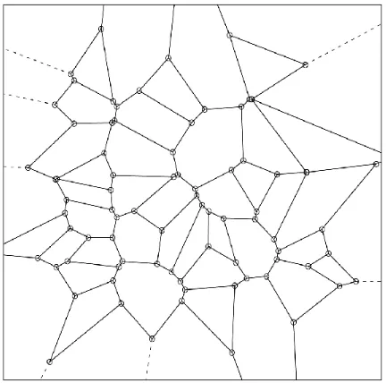
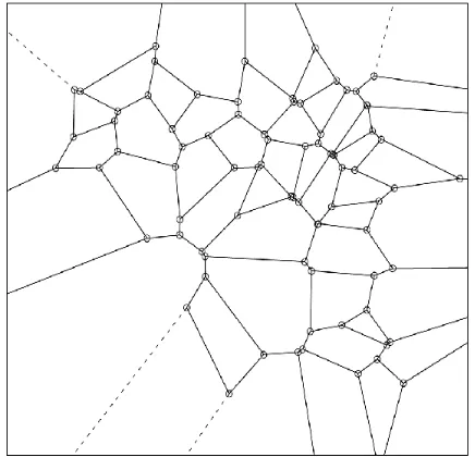
xand y are Cartesian coordinates of generated points. For each given point pattern, we randomly generated 30 instances containing 49 points in each. Then, Voronoi diagrams were formed for each instance upon the gener-ated points based on the above steps (Figures 2 and 3). The tripack package (Renka, 1996) in R was used to aid the generating process.
Figure 3: Simulated landscapes with 49 stands using Voronoi diagram method with an initial spatial point distribution ofp ∼ x2+y2.
2.5 Random Graphs A random graph is defined as a graph generated by a random process, often composed bynvertices and edges between them at random (Bol-lob´as, 2001). It is also very common in the forestry research to use a random graph to represent forest land-scape in a planar fashion, with vertices representing stands and edges representing the existing adjacency re-lationship between two stands. We took a different ap-proach, where there is a probability that any two nearby vertices may (or may not) be connected. The resulting set of random graphs was generated using the following steps:
1) Generatenrandom points;
2) Connect any two of the verticies based on a pre-defined probability.
In our study, we pre-defined five different probabil-ities, which are 0.02, 0.04, 0.06, 0.08, and 0.10. For each of these five probabilities, we generated 30 random graphs. The igraph package (Csardi and Nepusz, 2006) in R was used as the generating tool. Each of those ran-dom graphs contained 49 vertices, which represented the 49 forest stands. The physical distance between random points in these graphs has no influence on the resulting size of the management units, and the key data from these graphical representations is the spatial layout and resulting set of adjacency relationships. Since nearby edges may not be connected, these graphs are not neces-sarily planar, nor are they meant to describe or illustrate in a planar fashion the forested landscape. They are only used to locate adjacency relationships between vertices,
and thus not meant to be visualized as a set of forest polygons on a Euclidean surface. Further, since there is a probability that any two vertices may (or may not) be connected, the resulting graphs are not complete bi-partite graphs (or ”planar graphs,” or ”utility graphs”), where the graph(s)K3,3 exists as a minor graph.
All the stands in the gridded landscapes, the Voronoi landscapes, and the random landscapes generated in this study had the same non-spatial attributes, i.e., the stand size, timber volume productions in each time period, as the stands in the Daniel Pickett landscape. In other words, non-spatial attributes, as a complete package, were randomly assigned to generated polygons, whereas the actual size of polygons was irrelevant in this anal-ysis. Each of these new landscapes can be viewed as a ”reshaped” and ”rearranged” version of the Daniel Pick-ett forest. Therefore, valid comparison analysis can be carried out.
2.6 Problem Formulation A typical spatial forest planning problem was formulated and applied to the different representations of the forest landscape. The objective of this problem was to maximize the total tim-ber volume. To simplify the problem, we chose to have a planning horizon of three decades. The major con-straints included even-flow concon-straints and adjacency constraints. The mathematical formulations are as fol-lows:
Maximize
f =
3
t=1 49
i=1
ct
ixti (1)
Subject to
49
i=1
ct
ixti=Vt∀t (2)
β1Vt−1≤Vt≤βnVt+1 ∀t (3)
3
t=1
xt
i≤1∀t (4)
xt
i+xtj≤1∀ t, i j∈Ni (5)
Where:
β1= the lower bound in percentage for even-flow
con-straints
βn = the upper bound in percentage for even-flow
constraints
ct
i = timber volume produced from stand i in time
period t
i, j= an arbitrary harvested unit
Ni = the set of all harvest units adjacent to uniti
xt
i = decision variable, which equates 1 if
Vt= timber volume harvested in time periodt
Equation 2 is an accounting row that sums the volume scheduled for harvest during each time period. Equation 3 describes even-flow constraints, equation 4 indicates that a stand can only be harvested once during the plan-ning horizon, and equation 5 represents the adjacency constraints. These are standard pairwise adjacency con-straints that represent the unit restriction model of adja-cency among scheduled timber harvests (Murray, 1999). We applied this simple spatial forest planning problem to each of the generated forest landscapes and Daniel Picket Forest. The optimal solutions were obtained us-ing the ILOG- CPLEX student version problem solver.
3
Results
Summary statistics (maximum, minimum, mean, and standard deviation) of the optimal solutions, the CPU running time, and the number of adjacency constraints in one period were recorded for each of 30 simulated landscapes using the grid, Voronoi diagram, and random graph methods with different specifications, respectively (Table 1). The solution for the original Daniel Picket Forest with 49 stands was also solved with the same ob-jective and constraints for comparison purposes. The best solution for Daniel Picket Forest was 76,933 MBF and the CPU running time was 0.14 s. For simulated landscapes, although we had exactly the same 49 for-est stands, solutions varied considerably due to differ-ent adjacency relationships. The smallest average op-timal solution value was 72,100 MBF, when using the Voronoi diagram method with a spatial point distri-bution of p ∼ x2+y2, which was 6.3% less than
the original Daniel Pickett Forest. The largest average solution was 80,315 MBF for landscapes generated by random graphs with a probability of 0.02 for connect-ing two vertices (stands), which was 4.4% higher than the original Daniel Pickett Forest. For the Voronoi di-agram method, both the uniform and x2+y2
distri-butions had the average solution values less than their real-world counterpart data (72,259 MBF for uniformly distributed; 72,100 MBF for p ∼ x2+y2). This
in-dicates that adjacency restrictions in both distributions of Voronoi diagrams were much stronger than the ones in the original Daniel Picket Forest. The average opti-mal solution value for landscapes generated by the grid method (78,178 MBF) exceeded the average solution val-ues for the Daniel Picket Forest. This suggests that landscapes composed by grids with four interior neigh-bors had less restrictive power than the corresponding original landscape, and the number of adjacency rela-tionships (84 vs. 134) also gives evidence for this. For the random graph method, the average solution values decreased with the increasing probabilities of edge
con-nection. This is easy to comprehend since more edges suggest more adjacency constraints, and more adjacency constraints lead to lower solution values. When the edge probability equals 0.08, the average optimal solu-tion value (77,156 MBF) was closest to the comparison value (76,933 MBF).
Standard deviations of optimal solution values also differed greatly, with the smallest (274 MBF) for the random graph method withp= 0.02 (the least restric-tive), and the largest (1,310 MBF) for the Voronoi di-agram method based on uniformed distributions. It is interesting to note that the standard deviation followed an opposite trend relative to the optimal solution values. That is, with an increase in the average optimal solution value, the standard deviation decreased, which indicates that more adjacency restrictions might lead to greater variations. This also indicates that the processes which generated the better solutions were the least variable.
Average CPU running time also increased with an in-crease in the number of the adjacency constraints, which is what one may expect. On average, landscapes gener-ated by Voronoi diagram with a distribution ofx2+y2
required the maximum computing time (1.26 s), while the landscapes generated by random graph required the minimum computing time (0.17 s).
Compared with the original Daniel Pickett Forest, we found that although the average number of adjacency constraints were about the same (approximately 134) between Voronoi diagrams and the original landscape, the average optimal solution values for Voronoi diagram landscapes were much lower than those generated us-ing the original data (about 72,000 vs. 77,000 MBF), regardless of the initial spatial point pattern. The av-erage optimal solution values from random graph with
p= 0.08 most resembled the original Daniel Pickett For-est data, but it only had 95 adjacency constraints in one time period. Therefore, although adjacency constraints were closely related to the computing time, the solution values may still vary depending on the spatial structures and the method used to generate landscapes.
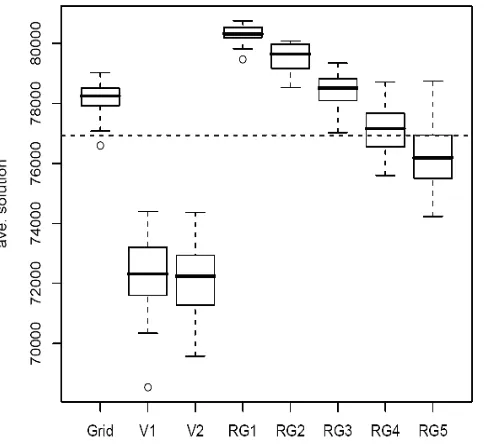
A boxplot (Figure 4) shows that the difference of mean solution values generated from each simulated landscape by three simulation methods. Tukey’s Honest Signifi-cant Difference’ (HSD) method was also used to perform multiple comparisons of optimal solution means among various simulation scenarios. Results show that only the pairs of V2 and V1 (p−value= 0.99) and RG3 and Grid (p−value= 0.92) were non-significant when α= 0.05 (Figure 5).
4
Discussion and Conclusions
pro-Table 1: Summary statistics of best solution values, CPU running time and number of adjacency constraints using three simulation methods respectively. CV = coefficient of variation
Grids Voronoi Diagrams Random Graphs Daniel Picket Uniform p∼x2+y2 p= 0.02 p= 0.04 p= 0.06 p= 0.08 p= 0.1 forest
Best avg. 78,178 72,259 72,100 80,315 79,550 78,443 77,156 76,205
76,933 solution max. 79,015 74,402 74,379 80,745 80,077 79,338 78,709 78,739
(MBF) min. 76,605 68,547 69,582 79,467 78,526 77,030 75,601 74,240 CV 0.65 1.81 1.65 0.34 0.56 0.69 1.00 1.41 avg. 0.68 1.22 1.26 0.17 0.27 0.42 0.91 1.23
0.14 Time max. 1.28 2.50 3.00 0.45 0.76 1.08 1.93 3.98
(s) min. 0.12 0.27 0.28 0.05 0.08 0.03 0.12 0.30 CV 55.88 49.18 57.94 64.71 66.67 69.05 60.44 67.48
avg. 84 133.8 133.9 23 46 70 95 115
134
number max. 84 137 137 35 56 82 114 137
of adj. min. 84 131 131 16 34 57 77 90
CV 0.00 1.27 1.19 17.39 13.04 10.00 9.47 7.83
Figure 4: Boxplot of the average optimal solution val-ues using three simulation methods and their different specifications (the horizontal dotted line is the average optimal solution for Daniel Pickett Forest); V1 refers to Voronoi landscapes generated with the initial uniformly distributed point pattern; V2 refers to Voronoi land-scapes generated with the initial spatial point distribu-tion ofp ∼ x2+y2; RG1-RG5 represents landscapes
generated by random graphs with edge probabilities of 0.02, 0.04, 0.06, 0.08, and 0.1, respectively.
−8000 −6000 −4000 −2000 0 2000
V2−V1 V2−RG5 V1−RG5 V2−RG4 V1−RG4 RG5−RG4 V2−RG3 V1−RG3 RG5−RG3 RG4−RG3 V2−RG2 V1−RG2 RG5−RG2 RG4−RG2 RG3−RG2 V2−RG1 V1−RG1 RG5−RG1 RG4−RG1 RG3−RG1 RG2−RG1 V2−Grid V1−Grid RG5−Grid RG4−Grid RG3−Grid RG2−Grid RG1−Grid
95% family−wise confidence level
Differences in mean levels of method
cess for improving objective function values, regardless of whether the researcher utilized heuristic approaches or exact mathematical approaches. However, this re-search provides a unique insight from a different per-spective, and illustrates how the hypothetical landscapes themselves, and the corresponding simulation methods for generating them, can be important considerations in evaluating solution processes designed for optimal har-vesting plans. As a result, the design of the hypothetical landscape is something one should consider in research regarding spatial forest planning issues. While 49 stands were used as an illustration of how the spatial layout may affect forest planning solutions, and while a larger num-ber of stands may seem appealing to illustrate other re-sults, we believe the conclusions from this study remain valid.
As detailed in the paper, we demonstrated how to use three different simulation methods (grids, Voronoi diagrams, and random graphs) to generate forest land-scapes with adjacency relationships. Generating grids is the most common method for simulating forest land-scapes, and in many cases, each cell represents one ho-mogenous stand. However, since each interior cell in a grid is restricted to having exactly four (sharing a com-mon edge) or eight (sharing a comcom-mon node) neighbors, such regularity is likely to prohibit its ability to resemble the real-world landscape to a useful extent.
Random graphs have also been introduced in some of the forest literature as an illustration of relationships among stands. Usually, such illustrations contain less than ten stands, and most were drawn by hand. Con-trary to the grid method, the greatest advantage of using random graph method lies in its above average ability to generate forest landscapes with variations in adjacency restrictions among the stands. The disadvantage lies in its poor visual quality. As the number of adjacency re-lationships increase, a clear layout of a random graph becomes rather difficult to visualize. Such low visual ability may hinder further analysis on characteristics of spatial landscape patterns, and thus impair the feasibil-ities of resulting planning solutions.
Landscapes generated by Voronoi diagrams represent a trade-off between the grid and random graph methods. They provide a relatively good visual construct, and also have a certain level of flexibility since one can control the initial spatial point pattern for each Voronoi diagram. However, since our results showed that strong adjacency restrictions existed in the Voronoi diagrams used in this study, we recommend that the Voronoi graph method be used to only represent relatively clustered landscapes as opposed to dispersed landscapes.
Each landscape generation method has its limitations. Both grids and Voronoi diagram methods can only gen-erate convex polygons, where the shape of real stands
can appear as either convex or concave. And the ran-dom graph method is likely to produce graphs that are not planar. Forest researchers should be aware of these limitations when choosing the appropriate method to generate the hypothetical landscapes. There also ex-ist other ways to generate planar landscapes, e.g., us-ing the MakeLand program (McDill and Braze, 2000), in which random points are first generated, then con-nected by arcs, and finally intersected arcs are removed based on certain specified rules. With any process, what we ultimately need for a landscape simulation in a harvest scheduling context are polygons (management units) and their associated adjacency relationships.
From our simulation study, we found two interesting points worthy of discussion. First, as one may surmise, adjacency constraints have a negative effect on the so-lution values (assuming the objective is to maximize an economic or commodity production goal). That is, the more the adjacency constraints one has in a spatial forest planning problem, the lower the objective values we may obtain. In general, this statement holds true, however our results also found that even with the same number of adjacency constraints, the solution values varied widely. That is to say, in a spatial context, not only the number of the adjacency constraints, but also how the adjacency relationships are set up among the stands affects the so-lution values. Although this point may seem obvious, it is not trivial. This effect caused by the spatial layout of adjacency relationships may easily be overlooked be-cause it is difficult to quantify the patterns of different adjacency relationships. The second point worth noting is also related to the adjacency constraints. We found in our study that the standard deviation of solution val-ues seems to increase with an increasing number of ad-jacency constraints. Combined with the first point, in the future forest planning researchers should be aware that different landscapes (spatial layout, per se) may result in significantly different planning solution values, especially when the number of adjacency constraints is relatively large.
can provide forest researchers a better understanding of different landscape generation methods and serve as a starting point for the future research.
Acknowledgements
We appreciate and value the constructive comments provided by the three anonymous reviewers of this manuscript.
References
Barrett, T. 1997. Voronoi tessellation methods to de-lineate harvest units for spatial forest planning. Canadian Journal of Forest Research. 27: 903–910.
Bollob´as, B. 2001. Random Graphs, 2nd Edition. Cambridge University Press. Cambridge, United Kingdom.
Bettinger, P., and J. Sessions. 2003. Spatial forest planning: to adopt, or not to adopt? Journal of Forestry. 101(2): 24-29.
Bettinger, P., J. Sessions, and K. Boston. 1997. Using tabu search to schedule timber harvests subject to spatial wildlife goals for big game. Ecological Mod-elling. 94: 111–123.
Chen, B.W., and K. van Gadow. 2002. Timber har-vest planning with spatial objectives, using the method of simulated annealing. Forstwiss. Cen-tralbl. (Hamb.). 121: 25–34.
Crowe, K., J. Nelson, and M. Boyland. 2003. Solving the area-restricted harvest-scheduling model using the branch and bound algorithm. Canadian Journal of Forest Research. 33: 1804-1814.
Csardi, G., and T. Nepusz. 2006. igraph Refer-ence Manual. Last accessed on Feb. 15, 2010 on http://igraph.sourceforge.net/doc/igraph-docs.pdf
Davis, L.S., K.N. Johnson, P.S. Bettinger, and T.E. Howard. 2001. Forest Management. Fourth edi-tion. McGraw-Hill. New York.
Gunn, E.A., and E.W. Richards. 2005. Solving the adjacency problem with stand-centred constraints. Canadian Journal of Forest Research. 35: 832-842.
Kurz, W., S. Beukema, W. Klenner, J. Greenough, D. Robinson, A. Sharpe, and T. Webb. 2000. TELSA: The Tool for Exploratory Landscape Scenario Anal-yses. Computers and Electronics in Agriculture. 27: 227-242.
McDill, M.E., and J. Braze. 2000. Comparing adja-cency constraint formulations for randomly gener-ated forest planning problems with four age-class distributions. Forest Science. 46: 423-436.
Murray, A.T. 1999. Spatial restrictions in harvest scheduling. Forest Science. 45: 45-52.
Murray, A.T., and R.L. Church. 1995. Measuring the efficacy of adjacency constraint structure in forest planning. Canadian Journal of Forest Research. 25: 1416-1424.
Nalle, D.J., J.L. Arthur, and C.A. Montgomery. 2005. Economic impacts of adjacency and green-up con-straints on timber production at a landscape scale. Journal of Forest Economics. 10: 189-205.
Okabe, A., B. Boots, K. Sugihara, and S. Chiu. 2000. Spatial Tessellations: Concepts and Applications of Voronoi Diagrams. John Wiley and Sons, West Sus-sex, England.
Renka, R.J. 1996. Algorithm 751: TRIPACK: a con-strained two-dimensional{Delaunay}triangulation package. ACM Transactions on Mathematical Soft-ware. 22: 1-8.
Thompson, M.P., J.D., Hamann, and J. Sessions. 2009. Selection and penalty strategies for genetic algo-rithms designed to solve spatial forest planning problems. International Journal of Forestry Re-search doi:10.1155/2009/527392 14 pages
T´oth, S.F., and M.E. McDill. 2009. Finding efficient harvest schedules under three conflicting objectives. Forest Science. 55: 117–131.
Van Deusen, P.C. 2001. Scheduling spatial arrange-ment and harvest simultaneously. Silva Fennica. 35: 85–92.