A Petri Net based Method for Analyzing
Schedulability of Distributed Real-time
Embedded Systems
Liqiong Chen
Department of Computer Science and Engineering, East China University of Science and Technology, Shanghai, China Email: [email protected]
Zhiqing Shao, Guisheng Fan and Hanhua Ma
Department of Computer Science and Engineering, East China University of Science and Technology, Shanghai, China Email: [email protected], [email protected], [email protected]
Abstract—As computer systems become increasingly internetworked, a challenging problem faced by researchers and developers of distributed real-time and embedded (DRE) systems is devising and implementing an effective shedulability strategy that can meet real-time requirements in varying operational conditions. In this paper, an extended Place-timed Petri nets (EPdPN) is proposed for schedulability analysis in DRE systems. First, we can capture important features of DRE systems and describe them by the semantic model. Second, the key component in DRE systems such as task, the relations between task, communication between module and resource et al. can be modeled by using EPdPN. Third, we present the concept of greatest concurrent set and convert schedulability problem into the analysis of state graph by using proposed algorithm, which can work out the feasible solution of scheduling in DRE systems. Finally, a specific example is given to simulate analytical process by using EPdPN, the results show that the method can be a good solution to analyze the schedulability of DRE systems.
Index Terms—Distributed real-time and embedded system, Petri nets, schedulability, state graph, communication
I. INTRODUCTION
Schedulability is a key challenge in the analysis of distributed real-time embedded (DRE) systems. Major design parameters that influence schedulability include realtime properties, such as task execution times and communication delays [1, 2]. Basically, in a DRE system, if time constraints are not met, the consequences can be disastrous, including great damage of resources or even loss of human lives. For example, a brake-by-wire system in a car failing to react within a given time interval can result in a fatal accident [3].
Therefore it is useful to analyze time constraints of DRE systems early in the lifecycle. Despite recent
advances in DRE systems development, however, there remain significant challenges that make it hard to develop large-scale DRE systems for domains that require hard timing constraints. The key unresolved challenges include the lack of formal methods for effectively modeling, integrating, and verifying.
To address these challenges, We propose an Extended Place-timed Petri Nets (EPdPN) model and introduce dual priority to transition. We describe the tasks and the relation between task of DRE systems in detail and convert schedulability problems into analyzing reachability of EPdPN model. In particular, we abstract communication process as a non-preemptive task, and using EPdPN model to characterize scheduling mechanism and time delay of communication process. Finally, we propose the concept of greatest concurrent set, and give a heuristic algorithm to compute feasible scheduling, the algorithm is realized by constructing part of state graph, thereby reducing the complexity of computation.
The remainder of this paper is organized as follows. Section 2 presents the definition and semantics of EPdPN model. Section 3 shows how EPdPN can be used to model DRE systems. Section 4 proposes the concept of greatest concurrent set and gives a heuristic algorithm for computing feasible schedule. In section 5, a specific example is given to simulate the modeling and analysis process. Section 6 presents some related works while section 7 is conclusions.
II. COMPUTATION MODEL
Petri net [4] is a mathematical formalism, which allows to model for the features present in most concurrent and real-time systems, such as timing constraints, synchronization mechanisms, and shared resources, etc. According to the features of DRE systems, we will use EPdPN to establish a suitable static scheduling model in this paper.
Definition 1: A Petri net is a 5-tuple, PN = (P, T, F, W, M0), where [4]:
(1) P = {p1, p2, ..., pn} is a finite set of places, n≥ 0; (2) T = {t1, t2, …, tm} is a finite set of transition, m≥0
and P∪T ≠∅ , P ∩T = ∅;
(3) F ⊆ (P × T) ∪ (T ×P) is a finite set of directed arcs; (4) W : F→ N*, N* is a set of non-negative integer, which is called the weight of arc;
(5) M0 : P → N*, M0 is the initial marking, which represents the initial state of system.
Definition 2: A 3-tuple ∑=(PN;C,Pr) is called Extended Place-timed Petri nets (EPdPN) model if:
(1) PN is a Petri net, which is called base Net of ∑; (2) C:P→N* is time function of place, C(Pj)=cj represents the token in Pj can not be used during the time from reaching the place to cj ; C is called delay time of place.
(3) Pr:T→(N*×N*) is priority function of transition, Pr(ti)=(αi, βi), and αi,βi are called primary and secondary priority of ti.
In this paper, the firing of transition in EPdPN model is instantaneous and the transitions called are determined by its priority. By default, the delay time of place is 0; the priority of transition is (0,0). The time units can be set according to specific circumstances.
In the modeling for DRE systems, its function is composed by a serious of interconnected tasks, which are mapping into transition, and the message transfer between tasks are characterized by place and its token. The distribution of token in each place at ∑ is called the marking of EPdPN, denoted by M. The marking M(p) denotes the number of tokens in the place p. M=Ma∪Mu, where Ma is the available tokens of M, Mu is the not available tokens of M; for any x∈(P∪T), we denote the pre-set of x as ●x={y|y∈ (P∪T)∧(y,x)∈F} and the post-set of x as x●={y|y∈ (P∪T)∧(x,y) ∈F}.
Because the tokens in EPdPN model including time factor, only using marking can’t describe the state of model. In order to better characterize time properties of model, we introduce the concept of wait time to describe the state of EPdPN.
Definition 3: Let EPdPN reaches marking M at time θ, the place Pi has j tokens in marking M, Pik is the kth token of Pi. Vector TS(Pi)=(TSi1,TSi2,……,TSij) is the wait time
of place Pi, where TS(Pik)= max{ci-(θ-ξk),0}, ξk is the time that token Pik generated. TSik is the wait time of
token Pik.
TSik=m presents that the system must wait m time units
before using token Pik. TS(Pik)= 0 represents the token is
available. Recorded TS(M) as wait time set of places under marking M.
Definition 4: A pair S = (M, TS) is called a state of ∑. Where M is marking, which describes the distribution of resources; TS(M) is the time stamp of marking M, which depicts time properties of system.
Initial state S0=(M0,TS0) where TS0 is a zero vector, i.e., all tokens are available in the initial state. Two ways can be used to change state:
(1) time elapse, at the time θ+ω (θ is the time reach the state S and ω > 0), because the wait time of tokens have changed which makes the model reach a new state S′, denoted by S[ω>S′.
(2) transition firing, the firing of transition ti will generate a new marking, thus the model will reach a new state S′, denoted by S[ti>S′.
S[ω>S′
and S′[ti>S′′ are denoted by S[(ti, ω)>S′′. Definition 5: Let Σ=(PN;C,Pr) is an EPdPN model, for transition ti∈T, if:
(1) ∀pj∈P:pj∈•ti→Ma≥W(pj,ti), ti is called strong enabled under marking M, denoted by M[ti>, all transitions that have strong enabled under marking M are recorded as set SET(M).
(2) ∀pj∈P: pj∈ •
ti→M≥W(pj,ti)∧Ma<W(pj, ti), ti is called weak enabled under marking M, denoted by M[ti≥, all transitions that have weak enabled under marking M are recorded as set WET(M).
If transition ti has weak enabled under marking M and at least pass through ω time units to be strong enabled, then ω is called the firing delay of transition ti under marking M.
Definition 6: Let Σ=(PN;C,Pr) is an EPdPN model, for transition ti∈T, the firing of transition ti is called effective firing iff it meets one of the following conditions:
(1) ti∈SET(M): αi≤min(αj)∧βi≤min(βk) where tj∈SET(M), tk∈U(ti)
(2) ti∈WET(M): SET(M)= ∅∧max(C( •
ti))≤max (C( •
tj)), tj∈WET(M)
All the effective firing transitions under the state S are denoted by FT(S).
Definition 7: A pair S=(M,TS) is the state of Σ, at the time θ+ω (θ is the time at reaching the state S, ω is the firing delay of transition ti), the model will reach a new state S′=(M′,TS′) by effectively firing transition ti, denoted by S[(ti, ω)>S′, S′ is called the reachable state of S, the computation of M′, TS′ are based on the following rules:
(1) Computing marking:
∀Pj∈●ti∪ti●, M′(Pj)=M(Pj)-W(Pj, ti)+W(ti, Pj) (2) Computing wait time:
First, adding time stamp to new generated marking: TS′(Pik)=ci, Pik is generated when firing transition ti;
Second, modifying the time stamp of tokens which are generated before the firing of transition ti: TS′(Pik)= max{(TS(Pik)-ω),0}, TS(Pik)≥0.
The computation of time stamp is mainly based on the generated time of token: for the newly generated tokens, the wait time is equal to the delay time of the corresponding place; if the token is generated before the firing of transition and not be removed; the corresponding wait time needs to be adjusted.
III. MODEL CONSTRUCTION
Bus Bus Controller
Task Set
Bus Controller Task Set
Bus Controller Task Set
N1 N2 Nn
…...
The EPdPN Model of TaskTKi A . DRE System Model
DRE systems can be regarded as a number of modules; each module also contains a number of partially ordered, serial or parallel implemented sub tasks [5, 6]. The function of DRE systems will be distributed to a number of interrelated embedded devices, each device is responsible for certain functions, and has certain autonomy, but relies on the computation of other embedded devices. The structural model of DRE system is shown in Fig. 1:
Among them, DRE system has n tasks; each task is composed by a series of interrelated sub tasks set and a bus controller. The effective and reliable communication between tasks is done by bus and bus controller. The communication process can follow different protocols, but we don’t focus on modeling communication protocol in this paper, therefore, we can assume the communication process between tasks is[7]: the task will send message to the cache of bus controller, and assign a priority to each message, the bus always send message which has high-priority; the system use nondestructive bus arbitration, when there are two nodes in the bus send message to the network at the same time, the low priority nodes will initiate to stop sending messages, while high-priority nodes can continue to send message. We can give following definitions based on the features of DRE systems:
Definition 8: DRE system model is a 7-tuple Ω={TK,N,RS,RL,TC,RT,SP}:
(1) TK is a finite tasks set;
(2) N={N1,N2,……Nn} is the collection of tasks set, Ni is the corresponding task set of module i;
(3) RS is a finite resources set;
(4) RL is the relation between tasks, which may be sequence, choice, parallel et al;
(5) TC:TK→(N*×N*×N*) is the time function of task, TC(TKi)=(ri,eci,di) , where ri,eci,di represent the release time, running time and deadline of task respectively.
(6) RT:TK→RS* is the resources function, whose function is to assign necessary resources to each tasks, RS* represents the multiple sets of resources, that is, a task can use multiple sources;
(7) SP:TK→N* is the static priority of task, SP(TKi)=SPi.
In this paper, we assume the tasks in a DRE system have the following characteristics:
(1) The task has time constraints including release time, running time and deadline.
(2) Static priority schedule is adopted to realize preemption.
(3) A task may also need other resources in addition to processor, such as variables or buffer; meanwhile each task has two ways to access the resources: exclusive access and sharing access.
(4) Each task can not suspend itself before completion. (5) The overhead of task switching can be neglected.
B. Modeling EPdPN
On the above DRE system model, we will abstract and model for tasks, communication between modules and resource, and forming the whole application according to the relation between tasks.
(1) Modeling Task TKi
According to the ways that task accesses resources, it can be divided into preemptive task and non-preemptive task. Preemptive task refers that the task can be interrupted by high-priority task during operating, while non-preemptive task refers that the task can not be interrupted by other tasks once operating; they must wait until the task automatic release resources after completion. Below we will model two types of task respectively.
Let the EPdPN model of task TKi is Σi=(PNi;Ci,Pri),, where PNi=(Pi,Ti,Fi,Wi,M0i). In the modeling of non-preemptive task (Fig.2(a)): Pi={Psi, Pdfi, Pdi, Pdmi, Pri, Pwi, Pei, PRSi}, Ti={tsi, tdi, tgi, tci}. cdi=di-eci explains if the time to deadline is less than the operation time of task, the overtime operation (tdi) will be executed. cwi=eci explains the operation of task requires eci time units. In the modeling of preemptive task (Fig.2(b)): Pi={Psi, Pdfi, Pdi, Pdmi, Pri, Pwi, Pfi, Pei, PRSi}, Ti={tsi, tdi, tgi, tci, tfi}. If task TKi has executed one time unit and high-priority task also competes its resources, TKi will release resources. The system will terminate and output the result after executing eci time units accumulatively. Table I lists the actual meaning of these transition and place. Among them, Place PRSi is modeling for reusable resources that task TKi required during processing, which can be added based on actual requirement. In order to simplify the model, we will model the preemptive task whose priority is (0,0) as non-preemptive task.
Based on the EPdPN model of task, we can allocate priority to the corresponding transition. In this paper, the allocation rules of priority are:
1) The primary priority of all transitions in Σi is equivalent to the priority of the corresponding task;
2) The secondary priority is divided into seven levels based on its importance: βfi=βci=0,βsi=1, βgi=4,βdi=6.
Figure 3. The EPdPN Model of Basic Relations
tfi
pbi
twbi
pwgbi
tgbi tcij
pbj
tsj
pbus
pcij,smij
Figure 4. TheEPDPNModel of Communication Process
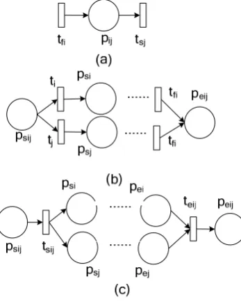
(2) Modeling Basic Relations
Assuming each task of DRE system has constructed the corresponding EPdPN model which is shown in Fig. 2. We will compose EPdPN model of each task by their relations. Suppose the EPdPN model of task TKi and TKj are Σi and Σj , the composed EPdPN model is Σ= (PN;C,
Pr), where PN=(P,T,F,W,M0). According to the basic relation between tasks (sequence, choice, concurrency), we can have the following mapping:
If the relation between task TKi and TKj is sequence, which means TKj can be fired only after executing task TKi, then we can add a place to connect the termination operation of task TKi and access resources operation of task TKj, which is shown in Fig. 3(a).
If the relation between task TKi and TKj is choice, which means only one task can be chosen to fire. As shown in Fig. 3(b), PSij is the common condition of TKi and TKj , while Peij is the output.
If the relation between TKi and TKj is parallel. The corresponding EPdPN model is shown in Fig. 3(c), where the function of Psij, tsij, teij and Peij is to control the parallel operation of tasks.
(3) Modeling Communication Process
In this paper, we abstract the communication process between modules as a communication task TKft, which is a 3-tuple (TKf,TKt,sm), where TKf, TKt, sm represent the message sender, receiver and required time respectively. We can construct the corresponding EPdPN model of task TKft, which is shown in Fig. 4. Σ=(PN;C,Pr), PN=(P,T,F,W,M0) where Pi={Pbi, Pwgbi, Pcij, Pbus, Pbj}, Ti={twdi, tgbi, tcij}. Let ccij=smij and the delay time of rest places is 0. Pbus is modeling for bus; Pwgbi represents the state that is waiting for getting tokens, while Pcij is the communication state. The primary priority of transition twdi, tgbi, tcij are equal to the priority of receiver while the secondary priority is: 2, 3, 5.
(4) Modeling Resource
In this paper, we assume the model doesn’t have memory limit when the tasks are executed, so memory is not considered as resource. For the sharing resources such as cache, processor, bus, and so on, we establish a place PRS. If the number of sharing resource is n, then we set M0(PRS)=n in the initial marking. For example, if task TKi need call the number of resources RS is w, we may set ●
tgi=●tgi ∪{PRS}, tci●=tci●∪{PRS}, W(PRS,tgi)=W(tgi,PRS)=w.
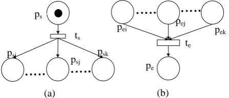
(5) Forming the Whole Application
The main purpose of this section is to form the EPdPN model of whole application based on the above model. The corresponding Model is shown in Fig. 5. First, we introduce the initial place Ps and transition ts which represent the beginning operation of the whole application, and ●ts={Ps}, ts●={Psi|●Psi=∅,i=1,2,……n},
●
Ps=∅, Ps●={ts}, M0(pS)=1; Second, we introduce the termination place Pe and transition te which represent the termination operation of whole application, and ●
ps
ts
psi
psj
psk
(a)
pe
te
pei
pej
pek
(b)
Figure 5. TheEPDPN Model of Start and End
Ⅳ. MODEL ANALYSIS
Schedulability is an important characteristic for guarantying the reliable of DRE systems. We first give the method for merging the firing of transition, and computing a feasible schedule of system.
In this section, EPdPN model is starting from initial state S0 and will generate new state through effectively firing enabled transitions, thus establishing a state space (known as state graph). The construction of EPdPN’s state graph is to outline the different firing sequences of transition, which make the complexity of computation exponential growth with the number of transitions increasing. Therefore, the concept of greatest concurrent set is introduced in this paper.
Definition 9: In the state S = (M, TS), transition ti, tj ∈FT(S) are called parallel, if:
(1) S[ti > S′→ tj ∈FT(S′); (2) S[tj > S′′ →FT(S′′)
Which is denoted as ti◊tj. Otherwise, we call transition ti, tj are conflict, denoted by ti⊗tj.
The firing of transition in the greatest concurrent set can not affect the firing of other transitions, denoted by S[H > S′. Let the number of transitions in H be n. We must compute n! states by using traditional analysis methods, however, we only need compute n-1 states by using the greatest concurrent set. So we can reduce the complexity of computation by using the greatest concurrent set.
We will introduce several special states before analyzing the schedulability of EPdPN model. Let ∑=(PN;C,Pr) is an EPdPN model, S=(M,TS) is a state of ∑:
(1) if ∃ pdmi ∈P which makes M(pdmi)=1, then S is called overtime state;
(2) if ∃ tdi ∈FT(S), then S is called dangerous state; (3) if M(pe)=1, then S is called normal termination state, denoted by SF.
Overtime state means that the operation can not be completed before the deadline, the model will reach overtime state when starts from the dangerous state; while the normal termination state is the state that all tasks have completed before the deadline; the other states in the system are called normal state.
Definition 11: Let the EPdPN model of Ω is ∑= (PN;C,Pr), then Ω is schedulable iff SF is reachable in ∑.
The model is schedulable if all tasks can complete before their deadlines, which is called a feasible schedule.
The feasible schedule is corresponding to a path from state S0 to SF in ∑.
Therefore, we can get the necessary part of state graph based on depth-first-search algorithm, thus getting the path. As the path is got from part of reachable graph, it may not be optimal.
The algorithm is based on the state graph of EPdPN model, which takes the initial state as root node, and
TABLEI. COMPUTING THE FEASIBLE SCHEDULING
Input: a bounded EPdPN ∑=(PN;C,Pr)
Output: the feasible scheduling for service composition
Schedule_Computer(S) 1: marking S
2: If (S==SF ) then 3: return FS;
4: Else if (FT(S)==∅) then
5: return false;
6: Else if all the child nodes of S have been marked then 7: top(State);
8: If ∃tgi∈FT(S) then 9: Top(FS); 10: ST=ST-ω;
11: Snew=Gettop(State); 12: End If
13: If Snew=S0 then
14: return false;
15: Else
16: Update_State(Snew); 17: End If
18: Else Update_State(S); 19: End If
Update_State(S) //Update feasible scheduling 20: calculate the greatest parallel set of S; 21: Seq_Computer(S,FT(S),H); 22: ST=ST+ω;
23: If ∃tgi∈δ then Push(FS,(Taski,……Taskj,ST)); 24: Push (State,Snew);
25: Sch_Computer(Snew); 26: End If
Seq_Computer(S,F,H) 26: If F=H then δ=H;
27: Elseoptional choose a transition ti 28: δ=H∪{ti};
29: F=F-ti; 30: Snew=S[(δ,ω)>; 31: End If
32: If Snewhas been marked then 33: Seq_Computer(S,F,H); 34: Else if ∃tdi∈FT(Snew) then 35: marked Snew;
Figure 6. TheEPDPN Model of Start and End
gradually computing every state in feasible schedule, we can do following operations for the current state S:
Step 1: If S is the normal termination state, then outputting the feasible schedule, otherwise go to Step 2;
Step 2: Computing firing set FT(S) of S, if FT(S) is empty set, then outputting error info, otherwise go to Step 3;
Step 3: If S is a dangerous state, then stepping back and updating feasible schedule;
Step 4: If S is a normal state, then computing the new state and continue to judge its state.
The algorithm is composed by three functions: function Compute_Schedule(S) is to determine to output or continuously operate based on current state; function Update_State(S) is to update the feasible schedule; while function Compute_Sequnce(S,F,H) is to compute next state. In order to get the result as early as possible in limited time, we must assure the model does not exist deadlock and loop. These two problems can be solved by modeling process in this paper. First, we assume tasks can be fired after obtaining all necessary resources, and it will release resource once completing(non-preemptive task) or running a time unit (preemptive task), thus breaking one of the necessary conditions of deadlock generated. While we don't consider task that has no time limit in modeling process, so there is no loop in this paper. In summary, the algorithm can be finished in limited time.
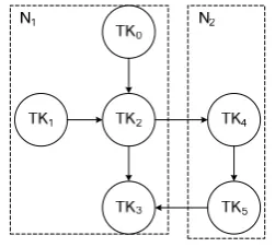
Ⅴ. EXAMPLE
In this section we illustrate the feasibility of analysis process by an example. Let Ω={TK,N,RS,RL,TC,RT,SP}, the system model as show in Fig. 6. where N1 = TK0, TK1, TK2, TK3; N2 = TK4, TK5, the special constrains are shown in Table II.
r1 = 1, the release time of other tasks is 0. Task TK1 and TK2 are competing for sharing resource RS01. Because the priority of task TK1 is 0, we can regard it as non-preemptive task during the process of modeling.
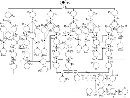
Among them, the communication refers the message sending between the modules. As the tasks in this system are relatively small, we can assume that task will idle once release the processor. So we could not consider the processor in the modeling of resource. Using the above modeling methods, we can construct the EPdPN model of Ω, which is shown in Fig. 7.
We can get a feasible schedule of Ω by using feasible
scheduling algorithm of Table I, the feasible scheduling computation steps of Fig. 7 are shown in Table III.
S, FS, ST, Snew represent current state, global time, new step of feasible schedule and new state respectively. We can draw that the model is scheduling by analyzing Table III, which is: (Tk0, Tk4, 0)→(Tk1, 1)→ (Tk0, Tk42, 4)→ (Tk2, 5)→ (Tk3, 9)→ (Tk35, 17)→ (Tk5, 18).
Due to space constraints, we only simulate for a simple example, but it sufficient to explain the accuracy and effectiveness of our proposed method for modeling and analyzing DRE systems. From the simulation process, we can get that EPdPN model can clearly express each component of DRE system. If we use general method for computing, the output of such a possible scheduling needs 34 steps, but here only using 15 steps, which explains the proposed heuristics algorithm in this paper can output results in limited time.
Ⅵ. RELATED WORKS
In recent year, there has been some related works used for DRE systems design including the non-formal methods and formal methods. The followings are related
TABLEIII.COMPUTING STEP
Step S FS ST Snew
1 S0 Null 0 S1=S0[ts > 2 S1 (Task0,Task4,0) 0 S2=S1[(tg0,tg4)>
3 S2 1 S3=S2[(tc0,1)>
4 S3 (Task1,1) 1 S4=S3[tg1>
5 S4 4 S5=S4[(tc1,tf4,3)>
6 S5 (Task0,Task42,4) 4 S6=S5[(tg0,tgb4)> 7 S6 5 S7=S6[(tc0,tc42,1)> 8 S7 (Task2,5) 5 S8=S7[(tf0,tg2)>
9 S8 9 S9=S8[(tf2,4)>
10 S9 (Task3,9) 9 S10=S9[tg3>
11 S10 17 S11=S10[(tf3,8)>
12 S11 (Task35,17) 17 S12=S11[tgb3>
13 S12 18 S13=S12[(tc35,1)>
14 S13 (Task5,18) 18 S14=S13[tg5>
15 S14 20 Send=S14[(te,2)>
16 Send
TABLEII. COMPUTINGTHEFEASIBLESCHEDULING
Task Running Time Deadline Priority
TK0 2 6 1
TK1 3 8 0
TK2 4 12 0
TK3 8 18 0
TK4 4 6 0
TK5 2 20 0
Sequence (TK1,TK2),(TK2, TK3),(TK0, TK3),(TK4,TK5) Communication (TK4,TK2)=1, (TK3,TK5)=1
non-formal methods: In [8, 9, 10], the authors proposed a global framework to support Distributed Real-time and Embedded application development based on methods,
such as pattern, component middleware and model-driven. And analyzed quality of service of Distributed Real-time and Embedded systems (energy, fault-tolerate, scheduling etc). But these methods only focus on high-level system, and lack the formal semantic of model. P. Paul et al [11, 12] used task graph to describe tasks and relations between tasks in DRE systems. More specifically, it discussed the schedulability analysis of DRE systems, and introduced several design optimization problems characteristic of this class of systems. However, the task graph lacks of rigorous mathematical foundation, so that the specification of its systems may contain ambiguous, vague, contradictory description of the requirement. Although the non-formal methods has made some corresponding results in the design of DRE systems, but they may cause some of the semantic ambiguity, in order to solve this problem, there has been some formal methods: G. Madl et al [13, 14 ] used Time Automata (TA) to model various components of the non-preemptive real-time distributed embedded systems and converted the system scheduling problem into TA state reachability. As the TA model implied the existence of global clock, it unfits for modeling the Distributed Systems. In [15, 16] used the time extended of Vienna Development Method (VDM++) to stipulate DRE systems, and used VDM
verification tools to verify the properties of system. However, comparing with other formal methods, the VDM may be more difficult to understand and grasp for
developers. A resource-based time Petri Net is proposed in [17] to model the DRE systems and analyzed the corresponding semantic, properties. But it didn't describe the communication between modules which is the key issue of DRE systems.
Ⅶ. CONCLUSIONS
The main contributions of this paper are: (1) attributing to the transition of Place-timed Petri Net to better describe the schedule strategy of the DRE systems by adding static priority; (2) summarizing the modeling steps of DRE systems in detail; (3) describing the characteristics against the EPdPN model and proposing the greatest concurrent set of the state, thus reducing the complexity of computation. Using this method for modeling and analyzing DRE systems has the following advantages: (1) with modular functionality and a high degree of reusability; (2) with a rigorous mathematical foundation, which can be easily used to analyze and verify the established model.
The study of DRE systems is still underway at present, the following two aspects are the main work in the next phase: (1) further improving this method, and considering the fault-tolerant of each task to guarantee the more
·
soundness of schedulability; (2) developing the corresponding tools to support modeling.
ACKNOWLEDGMENT
The research described here was partially supported by the NSF of China under grants No.60373075, the Science-Technology Development Foundation of Shanghai of China under Grant No.06dz15004-1.
REFERENCES
[1] X. Wang, Y. Chen, C. Lu, and X. Koutsoukos. “Fc-orb: A robust distributed real-time embedded middleware with end-to-end utilization control.” Journal of Systems and Software, 2007, 80(7). pp. 938–950.
[2] E. P. Freitas, M. A. Wehrmeister, C. E. Pereira, F. R. Wagner, E. T. Silva and F. C. Carvalho, “Using Aspect-Oriented Concepts in the Requirements Analysis of Distributed Real-Time Embedded Systems,” IFIP International Federation for Information Processing, Embedded System Design: Topics, Techniques and Trends. Boston, Springer.vol. 231, pp. 221-230, 2007.
[3] E. P. Carlos and C. Luigi, “Distributed real-time embedded systems: Recent advances, future trends and their impact on manufacturing plant control,” Annual Reviews in Control, 2007, 31(1). pp. 81–92.
[4] T. Murata. Petri nets: Properties, analysis and application. In Proceedings of the IEEE, volume 77, 1989, pp. 541–580. [5] K. Balasubramanian, J. Balasubramanian, J. Parsons, A. Gokhale, and D. C. Schmidt, “A platform-independent component modeling language for distributed real-time and embedded systems,” Journal of Computer and System Sciences, 2007, 73(2). pp.171–185.
[6] Z. Ying, D. TRobert, and C. Krishnendu, “Energy-aware deterministic fault tolerance in distributed real-time embedded systems,” In Proceedings of the 41st annual conference on Design automation. New York, ACM. pp. 550–555, 2004.
[7] G. Trombetti, A. Gokhale, D. Schmidt, J. Greenwald, J. Hatcliff, G. Jung and G. Singh, “An Integrated Model-Driven Development Environment for Composing and Validating Distributed Real-Time and Embedded Systems,” Model-Driven Software Development. Berlin Heidelberg, Springer. pp. 329-361.2005.
[8] W. Bin, W. Zhaohui, and C. Wenzhi, “Component model
optimization for distributed real-time embedded software,” IEEE International Conference on Systems, Man and Cybernetics, IEEE Computer Society. Washington. Vol.2. pp. 1158–1163, 2004.
[9] O. S. Unsal, I. Koren and C. M. Krishna, “Power-Aware Replication of Data Structures in Distributed Embedded Real-Time Systems,” Lecture Notes in Computer Science, Parallel and Distributed Processing. Berlin Heidelberg, Springer. vol. 1800. pp. 839-846. 2000.
[10]L. Patrick, B. Jaiganesh, D. C. Schmidt, T. Gautam, G. Aniruddha, and D. Thomas, “A multi-layered resource management framework for dynamic resource management in enterprise dre systems,” Journal of Systems and Software. 2007, 80(7). pp. 984–996,
[11]P. Paul, H. P. Kare, I. Viacheslav, and E. Petru,
“Scheduling and voltage scaling for energy/reliability trade-offs in faulttolerant time-triggered embedded systems,” In Proceedings of the 5th IEEE/ACM international conference on Hardware/software codesign and system synthesis. New York, ACM. pp. 233–238, 2007.
[12]P. Paul, E. Petru, P. Zebo, and P. Traian, “Analysis and optimization of distributed real-time embedded systems,” ACM Transactions on Design Automation of Electronic Systems. 2006, 11(3). pp. 593–625,
[13]G. Madl, N. Dutt and S. Abdelwahed, “Performance
estimation of distributed real-time embedded systems by discrete event simulations,” In Proceedings of the 7th ACM /IEEE international conference on Embedded software. New York, ACM. pp. 183–192, 2007.
[14]G. Madl, S. Abdelwahed and D. C. Schmidt, “Verifying Distributed Real-time Properties of Embedded Systems via Graph Transformations and Model Checking,” Real-Time Systems. vol. 33. pp. 77–100. 2006.
[15]V. Marcel, G. L. Peter, and H. Jozef, “Modeling and
validating distributed embedded real-time systems with vdm++,” In Proceedings of Formal Methods. Heidelberg, Springer-Verlag. pp. 147-162. 2006.
[16]M.Verhoef, and Larsen, “P.G.: Enhancing VDM++ for
Modeling Distributed Embedded Realtime Systems.,” Technical Report, Radboud University Nijmegen (March 2006) A preliminary version of this report is available on-line at http://www.cs.ru.nl/~marcelv/vdm/.
[17]Z. Haitao and A. YunFeng, “Time analysis of scheduling sequences based on petri nets for distributed real-time embedded systems,” In Proceedings of the 2nd IEEE/ASME International Conference on Mechatronic and Embedded Systems and Applications Washington. IEEE Computer Society. pp. 1–5. 2006
Liqiong Chen. She was born in 1982, Ph. D. candidate. Her research interests include distributed computing, embedded systems and formal methods.
Zhiqiong Shao. He was born in 1967, professor, Ph. D. supervisor, IEEE senior member, ACM member, China Computer Federation senior member. His research interests include software engineering, information security and formal methods.
Guisheng Fan. He was born in 1980, Ph. D. candidate. His research interests include service oriented computing, distributed computing and formal methods.