(DOI: 10.24874/jsscm.2017.11.01.08)
A radial 1D Finite Element for Drug Release from Drug Loaded
Nanofibers
M. Kojic1,2,3*, M. Milosevic2,4, V. Simic2, D. Stojanovic5, P. Uskokovic5
1Houston Methodist Research Institute, The Department of Nanomedicine, 6670 Bertner Ave.,
R7 117, Houston, TX 77030 e-mail: [email protected]
2Bioengineering Research and Development Center BioIRC Kragujevac, 6 Prvoslava
Stojanovica Street, 34000 Kragujevac, Serbia
e-mail: [email protected], [email protected]
3Serbian Academy of Sciences and Arts, 35 Knez Mihailova Street, 11000 Belgrade, Serbia
4Belgrade Metropolitan University, 63 Tadeuša Košćuška Street, 11000 Belgrade, Serbia
5Faculty of Technology and Metallurgy (FTM), University of Belgrade. 4 Karnegijeva Street,
11000 Belgrade, Serbia
e-mail: [email protected], [email protected]
*corresponding author
Abstract
The aim of this study was to investigate the release performance of an electrospun composite drug loaded nanofiber mat. Electrospun nanofiber mats are promising as drug carriers which offer site-specific delivery of drugs to a target in the human body and may be used for cancer therapy. The authors have formulated a simple radial 1D finite element, which is used to model diffusion within fibers releasing a drug to the surrounding medium discretized by continuum 3D finite elements. The numerical model includes degradation effects and hydrophobicity at the fibers/surroundings interface. For the purpose of experimental investigation, a poly(D,L-lactic-co-glycolic acid) (PLGA) implant has been created at the Faculty of Technology and Metallurgy, University of Belgrade. The radial 1D element provides accurate predictions of the diffusion process and serves as an efficient tool for describing transport inside the polymer fiber and surrounding porous medium; which is illustrated through numerical examples.
Keywords: Radial 1D finite element, diffusion, drug transport, emulsion electrospinning, PLGA implants
1. Introduction
83
that utilizes the electric force to drive the spinning process and to produce polymer fibers (Ramakrishna et al. 2005, Fong 2007, Greiner and Wendorff 2007), and is capable of producing fibers with diameters in the nanometer range (10–1000 nm). Nanofibers obtained by electrospining are structurally homogeneous and are unlikely to encapsulate bioactive agents as nano-scaled particles. Recently, electrospinning of emulsions has produced composite nanofibers with nano-scaled drug particles surrounded/coated by emulsifiers/surfactants and
impregnated in biocompatible and/or biodegradable polymers (Liao et al. 2008). Such a type of
composite nanofiber mats possesses the characteristics of a controllable drug encapsulation/release vehicle.
A composite nanofiber mat was prepared by electrospinning from an emulsion made of PLGA, Rhodamine B, sorbitan monooleate (Span-80), chloroform, N,N-dimethylformamide
(DMF), and distilled water, as in (Liao et al. 2008). PLGA has been well recognized for its
suitability in drug delivery due to its good biocompatibility and ability to achieve a complete drug release as a result of degradation and erosion of the polymer matrix. Furthermore, modeling the PLGA degradation and erosion is a prerequisite for drug release modeling, and mechanistic approaches are the most commonly employed (Sackett and Narasimhan 2011, Siepmann and Geopferich 2001). Accompanied and facilitated by PLGA degradation and erosion, drug release is significantly affected by the changing properties of the polymer matrix (porosity and PLGA MW) and such factors need to be captured in the diffusion drug transport.
The hydrophobicity of electrospun nanofiber mats could play an important role in the determination of their overall performances as tissue engineering scaffolds. While macromolecular hydrophilic drugs are limited by diffusion through the pore space, relatively smaller hydrophobic drugs could diffuse through both the PLGA matrix and the pore space (Zhu et al. 2015).
It is a challenge to adequately model by numerical methods the process of drug release from the fibers to the surrounding medium, with taking into account the transport conditions within the fibers (including degradation), in the medium, and at the interface between the fibers and the surroundings. The use of continuum elements for modeling fibers would require a huge effort for the finite element (FE) model generation and will lead to an enormous number of equations, therefore preventing the application to practical problems. In order to have a robust model, feasible for practical use, we here have introduced a radial 1D finite element which replaces a detailed modeling of fibers by continuum elements.
We further provide fundamental equations of the radial 1D element and the equation of degradation implemented into our model, and we also include the hydrophobic effects. At the end, using simple examples, we demonstrate the applicability of the numerical model.
2. Fundamental relations
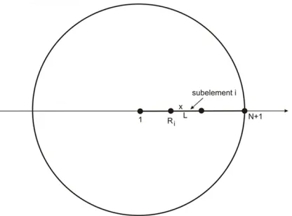
The diffusion domain in our model consists of fibers and surroundings filled with phenomenological fluid. The surroundings is modeled using 3D continuum elements, while the fibers are approximated by radial 1D elements. The radial elements can have 2 or more FE nodes. We further present equations for both of those cases.
1.1 2-node radial 1D FE
the fiber volume belonging to the common point. This belonging volume is equal to
π
R L
2 ,where
R
is the mean radius of the lengthL
belonging to the common point (it is (L1 +L2)/2 inFig.1). Further on, we neglect the diffusion along the fiber axial direction, therefore the diffusion occurs radially from the fibers to the surroundings.
With the above representation of the fibers and diffusion within the fibers, we are able to formulate a radial 1D finite element for the radial diffusion. At each common point of the fiber segments we introduce a radial 1D element which consists of two nodes, one in the middle of the fiber, and another at the fiber surface. Hence, node 1 is at the symmetry axis of the fiber, while node 2 is at the fiber surface. It is considered that node A of the 3D continuum (Fig. 1), closest to node 2 of the fiber, has the same concentration as node 2.
a)
b)
Fig. 1. Definition of 1D radial finite element
Now we can use the mass balance equations of the 2-node 1D FE element (Kojic et al. 2008) as:
(
)
1 J J 1 J J t
IJ IJ IJ IJ
M K C K C M C C
t + ∆ = − − t −
∆ ∆
(1)where matrices MIJ and KIJare:
0
2
R
IJ I J
M = πL N N xdx
∫
, ,
0
2 R
IJ I x J x
K = πL N
∫
N xdx (2)and
L
is the belonging length of the fiber segments (which is (L1+L2)/2 for the segment inFig.1).
Therefore, our radial 1D finite element has the volume which belongs to the considered common point of the fiber segments and represents a radial diffusion through that volume. We are using linear interpolation functions:
1 1 , 2
x x
N N
R R
= − = (3)
85
1, 2,
1
x x
N N
R
= − = − (4)
Now, we have:
11 22 12 21 2
0
2
Rfiber fiber
L
K
K
K
K
D
xdx
LD
R
π
π
=
= −
= −
=
∫
=
(5)where Dfiber is diffusion coefficient through the fiber volume. The “mass” matrix M is:
2
IJ I J
L
M =
π
L xN N dx∫
(6)and
11 1 1
0
2
2 2
12
R
M = πL xN N dx
∫
=π
LR2
12 21 1 2
2 2
12
R
L
M =M = πL xN N dx
∫
= π R (7)2
22 2 2
2 2
4
R
L
M = πL xN N dx
∫
= π R2.1 N-node radial 1D FE
We note that 2-node implies that the radial profile of concentration is linear, which is the first approximation of the true distribution. In order to have a nonlinear radial profile of concentration, and the corresponding (more accurate) flux from the fibers to the surroundings, we introduced radial elements with more than one node – i.e. with sub-elements, as shown in Fig. 2.
Fig. 2. Radial 1D element with sub-elements
1 1 , 2
x x
N N
L L
= − = (8)
with 1, 2, 1 x x N N L
= − = − (9)
Here we start with a local coordinate x=0 at the node on the left, with radius Ri. Matrices of
the element for this case are:
(
)
11 22 12 21 2
0
2 2
2 L
fiber i fiber i
L L L
K K K K D R x dx D R
L L
π
π
= = − = − = + = + ∫
(10)(
)
2IJ i I J
L
M = πL
∫
R +x N N dx (11)From (8) and (9) follows (after a corresponding derivation):
(
)
11 1 1
0 1 1 2 2 3 12 L i i
M = πL R +x N N dx= πLL R + L
∫
(12)(
)
12 1 2
0 1 1 2 2 6 12 L i i
M = πL R +x N N dx= πLL R + L
∫
(13)(
)
22 2 2
0 1 1 2 2 3 4 L i i
M =
π
L R +x N N dx=π
LL R + L
∫
(14)The calculation of initial concentration of drug in the fiber in case when using sub-elements is presented in the following subsection.
2.3 Determination of initial drug concentration at fiber nodes in case when number of sub-elements is greater than 2
The number of sub-elements affects the value of initial concentration that has to be prescribed at the fiber nodes at the start of an FE simulation. We further provide the derivation of the initial concentration based on the number of sub-elements. The mass of drug within a fiber segment is:
2
0 0
2
R
m= πLc
∫
x dx⋅ =RπLc (15)where
c
0 is the initial concentration of the impregnated drug. In case with n sub-elements, theconcentration within the first n-1 elements can be considered constant, while in the last
sub-element it is in the range from c0nto 0, where
0
n
c is the initial concentration which has to be
determined. In such case,the mass within a fiber segment, consisting of n sub-elements, is:
1
1
1 2 2 0 0 2
n
n
R R
n
n n n R x
m m m πLc − xdx πL c xdx
−
= + =
∫
+∫
(16)87 1 1 n n R R n − − = (17)
is the radius at the first node of the nth sub-element. The concentration along nth sub-element is
linearly changing according to the following equation:
1 0 1
(1 n ) n
x n x R c c R R − − − = − − (18)
Using (17) it follows from (18):
0
(
)
n x
n
c
c
R
x
R
=
−
(19)where
x
is changing fromR
n−1toR
, with R−Rn−1=R n/ . Now we have the followingequations: 2 2 1 0 1 n n n
m R Lc
n
π
− = 2 2 12 0 2 0
3 2
2 ( )
3 R n n n n R n n n
m Lc R x dx x dx R Lc
R n
π
− − π
= ⋅ ⋅ − ⋅ =
∫
(20)from which follows:
2
2
1 2 2 0
3 3 1
3
n n n n
n n
m m m R Lc
n π
− +
= + =
(21)
Using (15) and (21) we have finally:
2
0 2 0
3
3 3 1
n n
c c
n n
=
− + (22)
This is the value that has to be prescribed at each node of the sub-elements as the initial concentration, except at the node on the fiber surface - which is equal to zero.
2.4 Degradation and erosion effect on diffusion within PLGA nanofibers
In case when degradation and erosion is present in the model we assume that diffusion coefficient of the drug inside the fiber can be calculated according to (Zhu and Braatz 2015). The complete set of equations for describing the drug release through the PLGA polymer is summarized in Table 1 for clarity.
Drug Transport c D Me( w, ) c
t x φ x
∂ = ∂ ∂
∂ ∂ ∂
Effective diffusivity (1 ) 1
s l
e
D D
D
φ
κφ
φ κφ
− +
=
− +
Diffusivity in polymer solid 0
PLGA average MW molecular weight) ,0
w
k t
w w
M =M e−
Porosity change 2
(1 )(1 kt 2 kt)
e− e−
0 0
φ = φ + − φ + −
Table 1. Coefficient determined experimentally and computed by approximate expressions
Input parameters for the model with degradation and erosion effect are:
- De - effective drug diffusivity that is dependent on the evolving MW and porosity (ϕ)
- Ds - diffusivity in the polymer phase (Ds), - Dl - diffusivity in the liquid-filled pores (Dl)
- Mw - PLGA average MW
- Mw,0 - the initial weight-average MW,
- α=1.714 - according experiment
- k and k
w are degradation rate constants: k = kw = 2.5 x 10⁻⁷ s-1
- φ - porosity
- φ0= 0 - initial porosity of zero is used in the simulation
- P - drug partitioning between the liquid-filled pores and solid PLGA phase
- t - time
The practical procedure for including degradation and erosion effect in our model is as follows: Based on the current time t of simulation, according to the equation from Table 1, effective diffusion coefficient De is calculated and used as Dfiberfor radial 1D elements.
3. Model of PLGA implant
89
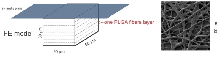
Fig. 3. Procedure for model generation. a) SEM images showing morphologies of the nanofiber mats, b) RReconstructed mesh of 1D fibers; c) FE model consisting of 1D fibers and
surrounding 3D FE mesh
By randomly duplicating and displacing the generated layer of 1D fibers into a longitudinal direction of the modeling domain, we can generate a realistic mat of fibers within any implant. Assuming symmetric conditions, we can model just one half of the implant. Also, assuming similar configuration of the fibers, and with the assumption that diffusion occurs in the radial direction, we can model just one part of the implant. So, the dimensions of our FE models are: 80x90x90 µm. 3D FE mesh is with 64512 nodes and 36864 elements, and the number of radial 1D elements within the system is related to porosity of the model and was in the range of 1895 - 7580.
Fig. 4. Configuration of the FE model, with symmetry conditions applied
We assume that the diffusion coefficient of Rhodamine B in pore space (a space between fibers) is as the one in water, and the diffusion coefficient of Rhodamine B within fibers (a fiber
with impregnated drug inside) is Dfiber = 4x10⁻¹⁰ cm2/s, which is taken from (Ruiz-Esparza G. et
al. 2014), which was approximately 104 times lower than the one in water. The time period of
simulation was 75 days. We used 15 times steps with 5 days each (15 x 5day = 75 days). The
boundary conditions of the model are: prescribed concentration C0 in fibers, and c = 0 at the
outer boundary of the implant (the boundary where mass release is measured).
4. Results
Fig. 5. Concentration change in PLGA fibers and 3D surroundings for diffusion process of Span-80/RhB complex within PLGA implant
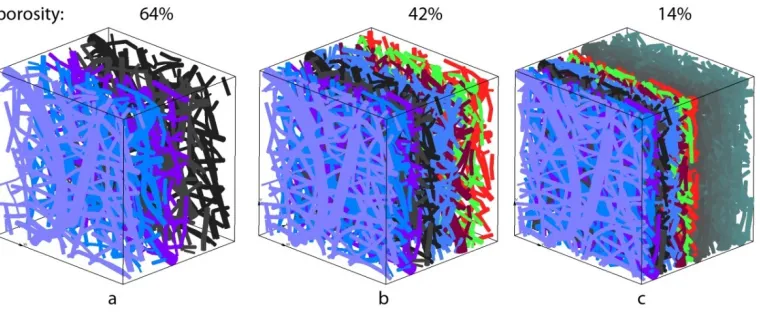
The porosity of implant is tuned by changing the number of reconstructed fiber layers within the diffusion domain, and by changing the thickness of one layer. The model with three different porosities is shown in Fig.6.
Fig. 6. Implant models with porosity of a) 64%; b) 42%; c) 14 %
The partitioning coefficient (P) reflects the hydrophobicity of the drug. The smaller the partition coefficient, the less water-soluble the drug is and the higher tendency of the drug to stay within the polymer solid. The effect of the partitioning coefficient is illustrated in Fig. 7 by fixing the other parameters (e.g. drug diffusivities in the polymer solids and aqueous phase).
91
simulations (Ziemys et al. 2011). Scaling functions takes into account the distance of a diffusion molecule from the nanofiber and the diameter of the molecule. It is obvious that for denser nanofiber mats molecules are constrained to movement, which is shown in Figure 7a.
a b
Fig. 7. Drug release vs. Time diagrams. a) Effects of model porosity; b) Drug partitioning on drug release
We have also used a smeared model (based on the formulation given in (Kojic et al. 2017; details are not presented here). In the smeared model we used the same parameters as for the above described detailed model: Diffusion coefficient of the diffusing drug within the PLGA
matrix is D = 0.04 µm2/s, and the other parameters are: Partitioning coefficient: P = 106,
Degradation rate constants: K = Kw = 2.5x10⁻⁷, Alfa = 1.714, Initial porosity = 0, D
plga = 10-8
µm2/s, and D
liquid = 0.04 µm2/s.
Fig. 8. Drug release profiles for constant diffusivity and for case with degradation
4. Conclusions
A radial 1D finite element is developed in order to model drug transport from drug loaded nanofibers. The 1D element incorporates partitioning and degradation effects which are important for modeling drug transport for drugs, used in practice, from commonly fabricated nanofibers. This concept offers computational modeling of drug transport within multilayered nano-implants used in tissue engineering, cancer healing and postoperative therapy.
Acknowledgements
The authors acknowledge support from Ministry of Education, Science and Technological Development of Serbia, grants OI 174028 and III 41007, and the City of Kragujevac.
References
Borden M, Attawia M, Laurencin CT (2002). The sintered microsphere matrix for bone tissue engineering: in vitro osteoconductivity studies. J Biomed Mater Res A 2002;61:421–9. Fong H (2007). Electrospun polymer, ceramic, carbon/graphite nanofibers and their
applications. In: Nalwa HS, editor. Polymeric nanostructures and their applications. Stevenson Ranch, California: American Scientific Publishers; p. 451–74.
Greiner A, Wendorff JH (2007). Electrospinning: a fascinating method for the preparation of ultrathin fibers. Angew Chem Int Ed;46:5670–703
Katti DS et al (2004), Bioresorbable nanofiber-based systems for wound healing and drug
delivery: optimization of fabrication parameters. J Biomed Mater Res B Appl Biomater
2004;70:286–296.
Kenawy ER et al. (2002). Release of tetracycline hydrochloride from electrospun poly(ethylene-co-vinylacetate), poly(lactic acid), and a blend, J Control Release;81:57–64. Kojic M, Filipovic N, Stojanovic B, Kojic N (2008). Computer Modelling in Bioengineering –
Theory, Examples and Software, J. Wiley and Sons.
Kojic M, Slavkovic R, Zivkovic M, Grujovic N, Filipovic N, Milosevic M (1998, 2017), PAK- FE program for structural analysis, fluid mechanics, coupled problems and biomechanics, Bioengineering R&D Center for Bioengineering, Faculty of Technical Science, Kragujevac, Serbia.
Kojic M, Milosevic M, Simic V, Koay EJ, Fleming JB, Nizzero S, Kojic N, Ziemys A, Ferrari M (2017), A composite smeared finite element for mass transport in capillary systems and biological tissue, Comp. Meth. Appl. Mech. Engrg., 324, 413–437.
Langer R (2003). Biomaterials in drug delivery and tissue engineering: one laboratory’s experience. Acc Chem Res;3:94–101.
Liao Y, Zhang L, Gao Y, Zhu ZT, Fong H (2008). Preparation, characterization, and encapsulation/release studies of a composite nanofiber mat electrospun from an emulsion containing poly (lactic-co-glycolic acid), Polymer (Guildf).Nov 10;49(24):5294-5299
Luo X, et al. (2012), Antitumor activities of emulsion electrospun fibers with core loading of hydroxycamptothecin via intratumoral implantation, Int J Pharm;425:19–28.
Park TG, Alonso MJ, Langer R (1994). Controlled-release of proteins from poly(L-lactic acid) coated polyisobutylcyanoacrylate microcapsules. J Appl Polym Sci;52:1797–807.
Ramakrishna S, Fujihara K, Teo W, Lim T, Ma Z (2005). An introduction to electrospinning and nanofibers. Singapore: World Scientific Publishing Co. Pvt. Ltd.
93
a cyclodextrin complex shell for potential site- and sequence-specific drug release,
Advanced Functional Materials, 24:30, 4753–4761.
Sackett CK, Narasimhan B (2011). Mathematical modeling of polymer erosion: Consequences for drug delivery. Int J Pharmaceut; 418:104–114.
Siepmann J, Geopferich A (2001). Mathematical modeling of bioerodible, polymeric drug delivery systems. Adv Drug Deliv Rev;48: 229–247.
Ziemys A, Kojic M, Milosevic M, Kojic N, Hussain F, Ferrari M, Grattoni A (2001). Hierarchical modeling of diffusive transport through nanochannels by coupling molecular dynamics with finite element method, Journal of Computational Physics, 230, 5722-5731. ISSN: 0021-9991. M21 – IF 2.485
Zhu X, Braatz RD (2015). A mechanistic model for drug release in PLGA biodegradable stent coatings coupled with polymer degradation and erosion. J Biomed Mater Res Part