www.theoryofcomputing.org
Interactive Proofs for
BQP
via Self-Tested Graph States
Matthew McKague
∗Received May 3, 2015; Revised June 1, 2016; Published June 18, 2016
Abstract: Using the measurement-based quantum computation model, we construct
in-teractive proofs with non-communicating quantum provers and a classical verifier. Our construction gives interactive proofs for all languages inBQPwith a polynomial number of quantum provers, each of which, in the honest case, performs only asingle measurement.
In this paper we introduce two main improvements over previous work in self-testing for graph states. Specifically, we derive new error bounds which scale polynomially with the size of the graph compared with exponential dependence on the size of the graph in previous work. We also extend the self-testing error bounds on measurements to a very general set which includes the adaptive measurements used for measurement-based quantum computation as a special case. These improvements allow us to apply graph state self-testing and measurement based quantum computation to build interactive proofs for all languages in BQP.
ACM Classification:F.1.3
AMS Classification:68Q15
Key words and phrases:complexity theory, quantum computing, interactive proofs, BQP
1
Introduction
We seek to find interactive proofs between quantum provers and classical verifiers, both limited to polynomial-time calculations. That is to say, we would like to have a procedure where a classical computer (the “verifier”), limited to a polynomial number of operations, can query a quantum computer
(the “prover”), also limited to a polynomial number of operations, and tap into its resources in order to perform some computation. Additionally, if the verifier unhappily interacts with a malicious quantum computer it should be able to detect this and abort the calculation, even if the prover has unlimited computational resources. To make the challenge less trivial, there should exist interactive proofs for problems that are harder than the verifier could solve by itself and ideally there should exist interactive proofs for any problem that the prover can solve by itself.
This problem is interesting for a variety of reasons. First, as a complexity theoretic question it has obvious value in further developing the theory of how powerful quantum computers are. From a practical computing point of view, it would be nice to know whether it would be possible to have cheap classical computers interact with large (and presumably more expensive) quantum “servers,” paying for services as required. Of course the users would like to know that they get their money’s worth, and interactive computations can confirm this. As well, from an experimental point of view, interactive proofs can be used to verify the operation of some experimental apparatus. This is of particular importance for quantum experiments since it may well be that, for large experiments, it is impossible (in practical terms) to classically compute what the predictions of the quantum model are, leading to questions about the falsifiability of the quantum formalism [3].
Clearly the set of languages recognizable by a poly-time classical verifier and poly-time quantum prover lies somewhere betweenPandBQPsince on one hand the verifier can ignore the prover, and on the other hand the verifier and honest prover together form a poly-time quantum machine. As well, there do exist interactive proofs for all ofBQPsinceBQP⊆PSPACEandPSPACE=IP[10,27], but the known constructions require the prover to solvePSPACE-complete problems. Constructions for particular problems are known ([16] for example) and of course anything inNPhas a trivial interactive proof. A general construction, however, has not yet been found.
One approach to solving the problem is to devise a method of detecting dishonest provers. Current techniques [1,4, 11, 12,13,15, 18, 20,22,23, 26] for probing the behavior of adversarial quantum systems all rely on entanglement and hence in order to make use of them we must introduce more provers. Reichardt et al. [26] considered the case of two provers. Here we will consider the case of a polynomial number of provers, but each limited to a single operation, and show that we can recognize all ofBQP with this model.
Thinking more broadly, we may look at different relaxations of the problem. One possibility is to grant the verifier some limited quantum capability. This approach is taken by Broadbent et al. [5] and Aharonov et al. [2].
Our construction uses two major components. One is self-testing and the other is measurement-based quantum computation. Self-testing allows us to confirm that the provers hold on to a graph state and perform certain measurements on this state when instructed to do so. Measurement-based quantum computation allows us to use these verified resources to perform the desired calculation.
1.1 Previous work
considered testing gates in the context of known Hilbert space dimension. Magniez et al. [11] combined the two approaches, allowing testing of entire quantum circuits. Further refinements, including simpler proof techniques and extension to complex measurements appear in [14] and [17]. Self-testing of graph states, critical for our application, appears in [15]. Miller and Shi [20] also give a general construction for self-testing states based on any XOR game.
These previous works all require additional assumptions. In particular, they assume that devices can be used repeatedly in an independent and identical manner in order to gather necessary statistics. As well, [11] assumes that certain states are in a product form. McKague and Magniez (in preparation) remove these assumptions for quantum circuits using techniques similar to those used here.
Stemming from a different heritage, Broadbent et al. [5] considered a semi-quantum verifier who only prepares single qubit states, and a fully quantum prover. They give a construction for an interactive proof for any language inBQP. Additionally, they describe an extension using two quantum provers and a classical verifier. Their construction uses measurement-based quantum computation. Improvements to the protocol appear in [8], while a rigorous proof of correctness for the classical verifier case appears in [8]. Aharonov et al. [2] also describe a semi-quantum protocol using a constant sized quantum verifier and a polynomial-time quantum prover.
In the context of quantum cryptography, Acín et al. [1] introduceddevice independent quantum key distribution.This model is very similar to that used here. However, rather than computation the goal is to expand a private shared key. From a physics perspective, Bardyn et al. [4] and McKague et al. [18] consider self-testing type entanglement tests from the perspective of Bell inequalities.
Most recently, Reichardt et al. [26] proved a very general result allowing two non-communicating quantum provers1along with a classical verifier to recognize all ofBQP. The core of their result is a self-test, using only two provers, for multiple EPR pairs and measurements. Using this tool they show how to test individual gates and perform measurements via teleportation. Finally, they combine the results to give an interactive proof for entire quantum circuits.
Measurement-based quantum computation, also known as one-way quantum computation or graph state computation, was introduced by Raussendorf and Briegel [24,25]. In this model of computation we begin with a graph state and perform measurements on each vertex, with the sequence of vertices and the measurement bases used determined by the calculation we wish to make. The outcome of the calculation is then derived from the measurement outcomes. One important aspect of the measurements is that they are adaptive—the measurement basis for a particular vertex can depend on the outcomes of measurements on previous vertices. This allows us to perform any calculation inBQP. The particular variety of graph-state computation that we use is due to Mhalla and Perdrix [19]. The advantage of this model is that it requires measurements in theX-Zplane only.
1.2 Contributions
Our main contributions are in improving self-testing. First, we modify the proof for the graph state self-test from [15], allowing a tighter error analysis. For graphs onnvertices the error in the state is upper bounded byO(√n)ε1/4(whereεbounds the noise in the experimental outcomes) rather thanO(2n/2)ε1/2
as in [15]. This exponential improvement in the error scaling innmakes it possible to self-test with a
polynomial number of trials to achieve a constant error. We also analyze the error in the case of adaptive measurements, which are required for measurement-based quantum computing. Additionally we extend the graph state test toX-Zplane measurements in order to achieve universal computation. Finally we show how to use the self-test in order to test the provers for honesty in the interactive proof scenario. Combining this test for honesty with measurement-based quantum computation we achieve the following theorem:
Theorem 1.1. For every language L∈BQPthere exists a polynomial time verifier V that on input x
interacts with a polynomial number of non-communicating quantum provers such that:
• If x∈L then there exists2 a set of honest quantum provers, each of which performs a single operation, for which V accepts with probability at least c=2/3.
• If x∈/L then, for any set of provers, V accepts with probability no more than s=1/3.
Along the way we also prove several results which may be of independent interest. In particular our error analysis for triangular cluster states (seeDefinition 2.12) can be applied to general graph states and stabilizer states enabling self-testing of these states with robust error bounds. As well, our error bounds for adaptive measurements are quite general, applying to general quantum circuits which incorporate the untrusted measurements performed by the provers.
While the Reichardt et al. [26] construction uses a constant number of provers, each of which runs in polynomial time, we use a polynomial number of provers, each of which runs in constant time (indeed, each prover only performs a single measurement). The advantage of our technique is that the provers are very easy to implement, requiring only the ability to measure in four different bases (once an appropriate graph state is prepared). Finally, there is a very nice conceptual advantage, which is thatthe measurement-based calculation that is performed is exactly what would be done with trusted devices, whereas the Reichardt et al. construction requires qubits to be teleported between the two provers at each gate.
1.3 Overview of construction
We can divide our interactive proof into two distinct units: the calculation and the test for honesty. The calculation is exactly the same measurement-based quantum computation that would be performed for trusted devices. The test for honesty is derived from self-testing.
We give some technical details of measurement-based quantum computation inSection 2.1. The procedure can be summarized as:
Procedure 1.
1. Prepare a universal graph state.
2. Perform measurements to obtain a computation-specific graph state.
3. Measure vertices in sequence, adapting bases according to outcomes from previous measurements.
2The honest provers and the verifier are, of course, members of a uniform set, i. e., a description of the verifier and provers
4. Calculate the final outcome.
In order to perform the computation we need the provers to share a graph state and be able to measure vertices. The verifier performs all the classical computation, including deriving the measurement patterns, the required graph state, and the final outcome.
Our main contributions lie in constructing a test for honesty. Here we must define some test such that if the provers were to cheat on the calculation then they will fail the test. Our test for honesty is based on the graph state self-test, originally presented in [15]. It allows the verifier to establish that the provers have access to high quality copies of the desired graph state andX andZPauli measurements. We give details for this test, including our improved proof inSection 3.1.
In addition, for the measurement-based quantum computation we also need measurements covering the entireX-Zplane. This is a simple extension of the graph-state test, which we present inSection 3.2. The graph-state test, with extensions, define a set of subtests, each of which the provers must pass. To administer the entire test, the verifier just chooses one of these subtests at random. If the provers actually hold the required graph state and perform the measurements faithfully then they will pass the test with high probability, and if their behavior deviates too much from the honest provers then they will pass with a lower probability. The gap is 1/poly(n)for a constant error bound and is calculated inSection 3.4.
With all of this in place we obtain a simple statement: if the provers deviate from the honest behavior by more thanδ (seeSection 2.5for a definition), then they will pass the test with probability at most
ctest−ε, whereε is a function ofδ andctestis the probability of honest provers passing the test. Hence if
the provers attempt to cheat we will catch them. The details are given inSection 3.4.
Having shown how to test whether the provers are honest, and how to perform the desired calculation, we must put these two components together to form the interactive proof. The structure is as follows: randomly either check for honesty or perform the calculation. The critical observation is that the queries to an individual prover look the same whether the verifier is testing or calculating. More specifically, every query that appears as part of a calculation also appears as part of the test for honesty. Henceprovers who attempt to cheat on the calculation can be caught by the test for honesty.
The final technical piece of the puzzle is to determine with what probability to test for honesty. We give the derivation inSection 4.
2
Technical introduction
In this section we present some notation and definitions used in the construction and proof.
2.1 Measurement-based quantum computation
Before we start, we define some standard quantum states operators. First, we have the states
|+i=√1
2(|0i+|1i), (2.1)
|−i=√1
2(|0i − |1i). (2.2) The Pauli operatorsX,Y andZare given by
X|xi=|x⊕1i, (2.3)
Z|xi= (−1)x|xi, (2.4)
Y|xi=iX Z|xi. (2.5)
We also have the Hadamard operator,H, given by
H|xi=√1
2(|0i+ (−1) x|
1i) (2.6)
and the controlled Pauli operators, given by
CTRL-X|xi|yi=|xiXx|yi=|xi|x⊕yi, (2.7) CTRL-Z|xi|yi=|xiZx= (−1)xy|xi|yi, (2.8) CTRL-Y|xi|yi=|xiYx|yi.
(2.9)
Note thatHX H=Zand(I⊗H)CTRL-X(I⊗H) =CTRL-Z. Further details about these operators, and quantum information in general, can be found in [21].
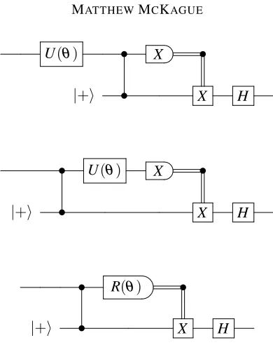
To understand how MBQC works, we will show how to turn a simple teleportation circuit into a circuit that applies a gate encoded in a measurement angle. Let us start with a basic teleportation circuit as inFigure 1. Rather than performing entanglement swapping with an EPR pair held in memory, as in the usual case, we entangle the input and output qubits directly using a CTRL-Xgate. The classical result of the measurement in theX basis is used to control aZgate, which applies a necessary correction. Direct calculation shows that the input state appears in the output register after the circuit is applied. In the second circuit inFigure 1, we convert the CTRL-Xgate to a CTRL-Zgate and two Hadamard gates. In the third circuit inFigure 1, the left Hadamard simply changes the initial state from|0ito|+i. We move the right Hadamard past theZcorrection, which then becomes anX correction gate.
Now suppose that we apply a unitaryUto the qubit as inFigure 2. For this construction we suppose thatU(θ) =exp(iθZ/2)so that it commutes with the CTRL-Zas in the second circuit ofFigure 2. Now
we can seeU as a modification of the measurement basis as in the final circuit. Since we originally measured in theX basis the new measurement basis will be in theX-Y plane of the Bloch sphere:
U†XU=R(θ) =cosθX+sinθY.
Next we consider how multiple teleportations work together. First we consider the case of two cascaded teleportations as inFigure 3. Using measurement anglesθ1andθ2, the overall unitary applied
by the circuit isHU(θ2)HU(θ1). In the second circuit ofFigure 3we have moved the second CTRL-Z
• X •
|0i Z
• X • |0i H • H Z
• X • |+i • X H
Figure 1: Three equivalent basic teleportation circuits. In the second circuit the CTRL-Xgate is replaced with a CTRL-Zgate sandwiched between two Hadamard gates. In the third circuit the left Hadamard gate changes|0ito|+iand the right Hadamard gate moves past theZcorrection, changing it to anX.
qubit. This induces aZcorrection on the third qubit, controlled along with theX correction. Finally, in the third circuit we incorporate theXcorrection into the measurement angle on the second qubit. Indeed, sinceX R(θ)X=R(−θ), the angleθ2becomes−θ2whenever anX correction is needed.
We have seen how to convertX corrections into changes in the measurement angle.Zcorrections are even easier to apply. SinceZR(θ)Z=−R(θ), aZcorrection corresponds to simply inverting the
output of a measurement.Figure 4shows howX andZcorrections together modify the behavior of the measurement.
So far our construction has the following features: we can apply a sequence of unitaries
HU(θn)· · ·HU(θ1)
to a qubit by repeatedly teleporting the qubit and varying the measurement angle used in the teleportation. The necessary corrections from the teleportation can be incorporated into subsequent measurement angles and outcomes, and all the entangling CTRL-Zgates can be pushed to the start of the procedure. Hence we can perform a single qubit circuit by first building a large entangled state using|+istates and CTRL-Z
gates, and then measuring the qubits in sequence, adapting measurement angles as we go. Note that the gatesHU(θ)form a universal set.
U(θ) • X • |+i • X H
• U(θ) X •
|+i • X H
• R(θ) •
|+i • X H
Figure 2: Three equivalent circuits combining a unitary with teleportation. In the second circuit the fact thatU(θ) =exp(iθZ/2)is diagonal means that it commutes with the CTRL-Zgate. In the third circuit
theU(θ)gate has modified the measurement basis toR(θ) =cosθX+sinθY.
pastXandZcorrections. This induces extra corrections which must be taken into account on subsequent measurements.
Now we have the complete picture. A calculation begins by preparing many|+istates and entangling them with CTRL-Z gates. Then they are measured one at a time, and measurements are adjusted to incorporateX andZcorrections as required.
The initial state, prepared by applying CTRL-Zgates to qubits in the|+istate, is called agraph state
(seeSection 2.4for a precise definition) and will play an important role in our results here.
Our construction will use a slightly different model of measurement-based quantum computation. Although the usual and most easily understood method utilizes measurements in theX-Y plane, we will instead use a different model, due to Mahalla and Perdrix [19], which requires onlyX-Z plane measurements. In particular they prove the following theorem:
Theorem 2.1(Mahalla and Perdrix [19]). Triangular cluster states are universal resources for measurement-based computation measurement-based on X -Z plane measurements.
• R(θ1) •
|+i • X • R(θ2) •
|+i • X
• R(θ1) •
|+i • • X R(θ2) •
|+i • Z X
• R(θ1) • •
|+i • • R(±θ2) •
|+i • Z X
Figure 3: Two cascaded teleportations. The first circuit teleports the first qubit to the third, applying
HU(θ2)HU(θ1). In the second circuit we have moved the CTRL-Z to the left past theX correction,
inducing aZcorrection on the third qubit, but allowing all the CTRL-Zgates to be applied before any measurements are made. Finally, sinceX R(θ)X =R(−θ)theX correction can be omitted in favor of a
change of measurement basis.
2.2 Operators, isometries, bit strings
We will frequently deal with a tensor product of operators over several subsystems. To make this easier we use the following notation:
Definition 2.2. Given some collection of operators{Mj : j=1. . .n}with Mj operating on the j-th subsystem, and a vectorx∈ {0,1}ndefine
Mx=
n
O
j=1
Mxjj. (2.10)
z •
x •
Z X R(θ) m
z •
x •
R(xθ) • mz
Figure 4: IncorporatingXandZcorrections into measurements. We haveX andZcorrections according to some previous measurement resultsx,z∈ {±1}. TheXcorrection is incorporated into the measurement as a change in the angle. TheZcorrection is incorporated by flipping the outcome of the measurement.
For an operatorMwe may also be interested in thecontrolledversion
Definition 2.3. LetMbe an operator onHA. Then the operator CTRL-M, which operators onH2⊗HA
is given by
CTRL-M|xi|ψi=|xiMx|ψi (2.11)
wherex∈ {0,1}.
Another set of objects that we will deal with frequently isisometries.
Definition 2.4. Anisometryis a linear operatorΦ:X→Ythat preserves inner products.
Isometries are a natural generalization of unitaries where the image space ofΦis not necessarily the same asX, and may in general have a larger dimension. As a concrete and pertinent example, adding an ancilla prepared in a particular state and applying a unitary are both isometries, as is their composition. Isometries are naturally extended to the dual space byΦ(hψ|) =Φ(|ψi)†and to operators
byΦ(|xihy|) =Φ(|xi)Φ(hy|), combined with linearity.
As we shall see, we will need to address the state spaces of provers individually, so we will need the concept of alocalisometry.
Definition 2.5. Alocal isometryonnsubsystems is an isometry of the form
Φ=Φ1⊗ · · · ⊗Φn (2.12)
whereΦj operates on the j-th subsystem only.
appropriate vector in the tensor product. That is to say,
Φ1⊗Φ2
∑
jxj
1
yj
2
!
=
∑
j Φ1
xj
1
⊗Φ2
yj
2
. (2.13)
By convention, we takeΦ1to meanΦ1⊗I2when applied to a state inH1⊗H2, and analogously for
other product spaces.
From this it is easy to derive the following properties of local isometries.
Lemma 2.6. LetΦ=Φ1⊗Φ2be a local isometry,|ψi1,2be a bipartite state, and M1be a local operator on the first subsystem. Then
Φ(M1|ψ1,2i) =Φ1(M1)Φ(|ψ1,2i). (2.14)
We make extensive use of bit strings. For ann-bit stringtthe j-th bit istj. Inner products of bit strings are given by
s·t=
n
∑
j=1sjtj. (2.15)
We will, at times, consider the inner product as an integer, and at other times as a bit (i. e., overZorZ2).
Where the difference is important we will specify. For example,t·ttaken overZgives the number of
ones intbut when taken overZ2it is the parity of the number of ones.
Finally, we define the bit string 1v to have a 1 only in the v position and zeros elsewhere, i. e.,
(1v)j=δv j.
2.3 Technical lemmas for estimation
We will need to make use of several easy technical results in our proofs. We collect them here for convenience.
Lemma 2.7. Let|ψiand|φibe normalized states. Supposehψ|M|ψi ≥1−α andhψ|N|ψi ≥1−β
where M2=N2=I. Then
|||ψi −M|ψi|| ≤
√
2α, (2.16)
|||ψi −MN|ψi|| ≤
√
2
√
α+pβ
. (2.17)
Further, if M is unitary and|ψ1iand|ψ2iare normalized states, then
|hφ|M|ψ1i − hφ|M|ψ2i| ≤ |||ψ1i − |ψ2i||. (2.18)
The first inequality is a straightforward applications of the definition of||·||. The second inequality is an application of the first, along with the triangle inequality. The last inequality is an application of the inequality||O|ψi|| ≤ ||O||∞|||ψi||2where we use the operatorO=hφ|M.
Lemma 2.8. Let t be an n-bit string. Then
∑
s∈{0,1}nIft=0 then the summand is always 1. Ift6=0 then half the stringsshave inner product 0 withtand the other half have inner product 1, so we get a sum with half the summands 1 and the other half -1.
Lemma 2.9. Let u∈ {0,1}nbe given and letAbe the adjacency matrix for a graph G= (V,E). Then 1
2n
∑
s∈{0,1}ns·u= u·u
2 , (2.20)
1 22n
∑
s,t∈{0,1}n
s·t= n
4, (2.21)
1 2n
∑
t∈{0,1}n
t·At= |E|
4 . (2.22)
For the first one, the average inner product of a vector withuis half the number of 1’s inu. The second computes this for an averageu, which hasn/2 1’s. For the last one,t·Atcounts the number of edges in the induced subgraph onSt ={v∈V|tv=1}.
Consider an edge(u,v). Then(u,v)appears in the induced subgraph onSt whenever both ends are in St, i. e., whentu=tv=1. This happens for a quarter of all bit stringst. Hence each edge is counted 2n−2 times for a total of 2n−2|E|.
Lemma 2.10. Let x∈ {0,1}n. Then
H⊗n|xi=√1
2n
∑
y∈{0,1}n(−1)x·y|yi. (2.23)
This is a standard result in quantum computing, and can be shown using induction onn.
2.4 Graph states
We assume that the reader is familiar with the basics of graph theory. A good resource is [7]. We now fix some notation for our convenience. LetG= (V,E)be a graph,n=|V|andu,v∈V. Theadjacency matrixAofGis a{0,1}matrix withAu,v=1 whenever(u,v)∈E and 0 elsewhere. Note thatA1vis a vector containing a 1 in positionufor each(u,v)∈E, and is hence the characteristic vector of the neighborhood ofv. AsubgraphofGis a graph with verticesV0⊆V and edgesE0⊆Esuch that all edges inE0 go between vertices ofV0. Finally, theinduced subgraphon a subsetS⊆V is the graph on vertices
Swhich has edges{(u,v)|u,v∈S,(u,v)∈E}. In other words, the induced subgraph is themaximal subgraphofGon vertices inS. Atriangleis a set of three vertices which are pairwise adjacent.
The graph state|Giis ann-qubit state, with qubits labeled by vertices, which is stabilized3by the operators
Sv=XvZA1v. (2.24)
That is,Sv hasX on vertexvandZon each of its neighbors and
Sv|Gi=|Gi. (2.25)
Equivalently,
|Gi=√1
2n
∑
x∈{0,1}n(−1)12x·Ax|xi (2.26) with the inner product overZ. To explain, let us write
x·Ax=
∑
u,v xu=1=xv
1u·A1v=
∑
u,v xu=1=xvAu,v. (2.27)
Now sinceAu,v=Av,u=1 whenever (u,v)∈E, we are counting edges. The summation and Aare symmetric, so we are double counting and we always get an even number (hence the 1/2 appearing in the exponent above). LetTx={v|xv=1}, then we are summing over all the vertices inTx, double counting the edges in the induced subgraph onTx.
For completeness we show that the above two definitions are equivalent by showing that|Gi is stabilized bySv:
XvZA1v|Gi= 1
√
2n
∑
x(−1)12x·Ax(−1)x·A1v|x⊕1vi (2.28)
=√1
2n
∑
x(−1)12(x⊕1v)·A(x⊕1v)±(x⊕1v)·A1v|xi (2.29)
where we have re-indexed the summation byx→x⊕1v. The±in the exponent of the−1 represents the fact that we only care about the parity of the exponent, so we can add or subtract as we please.
Now(1/2)(x⊕1v)·A(x⊕1v)is the number of edges in the induced subgraph onTx⊕1v. Meanwhile
(x⊕1v)·A1v=x·A1vsince 1v·A1v=0 (no vertex is adjacent to itself) andx·A1v counts the neighbors ofvthat are inSx.
There are two cases. First, ifv∈TxthenTx⊕1v does not containv. The subgraph onTx is obtained from the induced subgraph onTx⊕1v by addingvand all the associated edges—x·A1vof them—and the total number of edges in the induced subgraph onTxis
1
2(x⊕1v)·A(x⊕1v) + (x⊕1v)·A1v= 1
2x·Ax. (2.30)
In the other casev∈/Tx, so we obtainTxby removingvand all associated edges fromTx⊕1v, so
1
2(x⊕1v)·A(x⊕1v)−(x⊕1v)·A1v= 1
2x·Ax. (2.31)
Hence
XvZA1v|Gi= 1
√
2n
∑
x(−1)12(x⊕1v)·A(x⊕1v)±(x⊕1v)·A1v|xi (2.32)
=√1
2n
∑
x(−1)12x·Ax|xi (2.33)
We have shown that the operatorsSv stabilize|Gi. It is also easy to see that theSv operators are independent: any one cannot be obtained by multiplying together others. They also commute with each other. We then havenindependent, commutingn-qubit Pauli operators which stabilize a 1-dimensional space [9].
Operationally, graph states are constructed by beginning with the qubits in the state |+i⊗n and applying CTRL-Zgates on verticesu,vwhenever(u,v)∈E.
We can generalize the above argument as follows:
Lemma 2.11. LetAbe an n×n adjacency matrix and x,y be n-dimensional{0,1}-vectors. Then
(−1)12(x⊕y)·A(x⊕y)+(x⊕y)·Ay= (−1) 1 2x·Ax+
1
2y·Ay. (2.35)
Proof. We first do everything overZ. By linearity
(x+y)·A(x+y) =x·Ax+y·Ay+x·Ay+y·Ax. (2.36) SinceAis symmetricx·Ay=y·Ax. Thus, dividing everything by two and rearranging, we obtain
1
2(x+y)·A(x+y)−x·Ay= 1
2x·Ax+ 1
2y·Ay. (2.37)
Note that both sides of the equation will always be integer. Now
(−1)12(x+y)·A(x+y)−x·Ay= (−1) 1 2x·Ax+
1
2y·Ay. (2.38)
We only care about the parity of the exponents so we can make two small changes. First, the−becomes a+. Second, we can addy·Aysince it is always even and won’t affect the parity. Thus,
(−1)12(x+y)·A(x+y)+(x+y)·Ay= (−1) 1 2x·Ax+
1
2y·Ay. (2.39)
Finally, we can do the additions modulo 2 (+becomes⊕) since we only care about the parity. This gives the desired result.
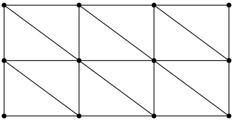
The graphs that we will mostly be concerned with aretriangular latticegraphs.
Definition 2.12. Anm×n triangular lattice graphhasmnvertices,{v(a,b)|a=1. . .m,b=1. . .n}where vertexv(a,b)is adjacent to verticesv(a+1,b),v(a,b+1),v(a+1,b+1),v(a−1,b),v(a,b−1)andv(a−1,b−1)when they
exist.
A small example is given inFigure 5.
2.5 Definition of “closeness”
Figure 5: Triangular lattice graph.
both the state and measurements). In fact, we will see that for the states and observables we use these are theonlyundetectable transformations that they can apply.
We can account for such transformations by allowing an arbitrary isometry which undoes these transformations and presents us with the required graph state plus some arbitrary ancilla state. We also allow for some noise by comparing states in the usual vector norm.
Definition 2.13. We say that a multi-partite (i. e., with more than one subsystem) state|ψ0iand
observ-ables{M0}are
ε-equivalent4to|ψiand{M}if there exists a local isometryΦand a state|junkisuch that for everyM
Φ(M0
ψ0)− |junkiM|ψi
2≤ε. (2.40)
Here we are thinking of “M” as both the ideal operation on|ψiand as a label for the operationM0.
Evidently this definition guarantees that the two systems behave like each other since isometries preserve inner products, and hence outcome probabilities. As we shall see, it is also a necessary condition for states and measurements to behave close to the ideal graph states andX-Zplane measurements. Hence any other definition we could choose is at most a different characterization of the errors and in the exact case is equivalent. The error bound used here has an operational meaning since we can quickly bound the error in outcome distributions from it.
There is one shortcoming of this definition, which is that it is impossible to test states or operators which contain any imaginary component in the ideal case (this restriction does not apply to the states and operators held by the provers, only to the ideal that we compare them to.) The simple reason is that the provers may apply a complex conjugation to everything without changing the distribution of their responses to the verifier. This transformation is not an isometry, and hence it is impossible to conclude that any system satisfies the above definition based on classical interaction alone. It is, however, possible to extend the definition to account for this case [17]. We do not need to use this extended definition here since all ideal operators and states in the Mahalla and Perdrix construction are real.
4It is easy to see that this relation is (in the exact case) transitive and reflexive, but it is also clearly not symmetric. Thus it is
2.6 Modelling the provers
An important argument in our work is that we can model the provers, even in the dishonest case, by a pure joint state held by the provers, and a collection of observables for each prover, one per possible query to that prover.
First, it should be clear that it is not a restriction to consider pure states. Any mixed state can be purified and the purification given to any one of the provers. This only increases the power of the provers by giving them additional information held in the purification.
Next, since our provers will only receive one query and respond with one message, we can model their actions by a measurement. Any pre-processing done before the measurement can be incorporated into the choice of measurement as can any post-processing. Further, since we are not making any assumptions on the dimension of the state held by the provers, their measurements can be taken to be projective and, since the provers will always respond with±1, the projectors can be combined into an observable without any loss of information or generality.
It is important to consider the view of a single prover during the protocol. They will receive one of four measurement settings, all of which appear in the test for honesty, but not all will necessarily appear as part of the computation. For settings that appear only in the test, the prover may decide to act honestly, but this will not affect the outcome of the computation. Let us say that setting 1 appears in both the test and the computation. The prover has no other information to act on, and so must measure some operator
M1. They may decide onM1based on the different distribution of measurement settings for the test and
the computation, but they are still left with a fixedM1to be measured when queried with setting 1. Thus the verifier can be sure that theM1measured during the test is the same as theM1measured during the
computation. What we need to prove, then, is that a strategy (state and measurement operators for each measurement setting) cannot both pass the test with high probability and bias the calculation.
3
Test for honesty
In order to develop a test for honesty we go through several steps. The first step is to develop a test for graph states. This is the foundation on which we build the test for honesty. After showing how we can verify that the provers hold onto a particular graph state we then show how to test measurements in the
X-Zplane. Adaptive measurements built on measurements in theX-Zplane are the next step. Finally, we put all of the tests together into a single test and show how the probability of passing this test relates to the amount of error in an adaptive measurement performed on the same state and using the same measurements.
3.1 Self-test for triangular cluster states
Theorem 3.1. Let G be a triangular lattice graph on n vertices with adjacency matrixAand letε >0.
Further, suppose that for an n-partite state|ψ0iwith local measurements Xv0 and Z0vwe have for each v∈V
ψ0S0v
ψ0
≥1−ε (3.1)
(where S0v=Xv0Z0A1v) and for each triangle T⊆V with characteristic vectorτ
−
ψ0X0τZ0Aτ
ψ0≥1−ε (3.2)
then there exists a local isometryΦand state|junkisuch that
Φ X0qZ0p ψ0
− |junkiXqZp|Gi ≤
2√p·p+2
√
2n+p|E|+n
(2ε)
1
4 (3.3)
for all p,q∈ {0,1}n.
We may interpretTheorem 3.1 as follows: for each triangular cluster state there exists a set of non-local correlations that uniquely identifies that graph state andX andZ measurements, up to local unitaries and additional ancillas.
The proof can be divided into several sections. The final goal is to construct an isometryΦand prove that it takes the state|ψ0iclose to the desired graph state. The construction for the isometry is given in
terms of theX0andZ0operators on each vertex. To bound the error we need to know how these operators behave and in particular whether they approximately anti-commute. This is done inLemma 3.2and
Corollary 3.3. In the ideal case we can use the stabilizers to showXv|Gi=ZA1v|Gi. InLemma 3.4we
show that this is approximately true for theX’s, which will allow us to convertX0s intoZ0s. With these estimations in place we then proceed with the proof ofTheorem 3.1.
3.1.1 Preliminary technical estimations
Our graphGis a triangular lattice, so every vertex lies in a triangle. For self-testing this gives a nice advantage, since it is particularly easy to show thatX0 andZ0anti-commute for vertices in a triangle.
Lemma 3.2. Let v∈V be a vertex in a triangle. Under the conditions ofTheorem 3.1,
Xv0Zv0
ψ0
+Zv0Xv0ψ0
≤4
√
2ε. (3.4)
Proof. First, letT={u,v,w}be a triangle containingv. The first part ofLemma 2.7, together with the conditions ofTheorem 3.1, tell us
S0x
ψ0−ψ0 ≤
√
2ε (3.5)
forx∈ {u,v,w}, and from triangleτ X 0 uX 0 vX 0 wZ
0A1uZ0A1vZ0A1w ψ0
+ψ0 ≤ √
2ε. (3.6)
Applying the second part ofLemma 2.7three times to combine these, we find
S 0 uS 0 vS 0 wX 0 uX 0 vX 0 wZ
0A1uZ0A1vZ0A1w ψ0
+ψ0 ≤4 √
TheZ0s operating on vertices outsideT all cancel since they appear inSx0 and inZ0A1xfor somex∈ {u,v,w}
and there are noX0operators outside the triangle. We are left with
(Xu0Zv0Zw0)(Zu0Xv0Zw0)(Zu0Zv0Xw0)(Xu0Xv0Xw0) ψ0
+ψ0
≤4
√
2ε. (3.8)
By commuting operators on different subsystems past each other, we can pair up and cancel theXx0 and
Z0xforx∈ {u,w}, resulting in
Xv0Zv0Xv0Zv0
ψ0+ψ0 ≤4
√
2ε. (3.9)
Rearranging by multiplying byZv0Xv0, we obtain our result.
Note that it is sufficient to consider a set of triangles that covers the set of vertices and hence
Theorem 3.1holds for all graphs in which each vertex is contained in a triangle. In fact, as in [15], it is
sufficient to consider one triangle or just one edge in a connected graph, but this will give a less robust result. Lemma 2 in [15] shows that ifXv0andZv0 approximately anti-commute, then so doXu0andZ0ufor some neighboruofv. Using this one can induct along paths to all vertices in a connected component. For our purposes this is unnecessary since all vertices lie in at least one triangle.
The above lemma can be generalized to products of operators, as in the following corollary.
Corollary 3.3. Let s,t∈ {0,1}n. Under the conditions ofTheorem 3.1,
X0tZ0s
ψ0
−(−1)s·tZ0sX0tψ0
≤4(s·t)
√
2ε, (3.10)
where s·t is taken overZ.
This can be seen by repeatedly applyingLemma 3.2, once for everyvsuch thatsv=1=tv, and using the triangle inequality. Ifsx=1 buttx=0, or vice versa, for somex∈V, then the single operator on vertexxcommutes with all other operators.
Now we consider the physical analogue of the stabilizer generators which are defined byS0v=Xv0Z0A1v. The conditions ofTheorem 3.1establish that they really are (close to) stabilizers of|ψ0i. Next we consider
products of these generators and show that they too almost stabilize|ψ0i.
Lemma 3.4. Let t∈ {0,1}n. Under the conditions ofTheorem 3.1,
X 0t ψ0
−(−1)12t·AtZ0Atψ0
≤(2(t·At) +t·t)
√
2ε, (3.11)
where t·At and t·t are evaluated overZ. Proof. First, byLemma 2.7we find
ψ0−
∏
v∈V tv=1
S0vψ0
≤(t·t)√2ε. (3.12)
The right term in the norm can be expanded as
∏
v∈V tv=1S0vψ0=
∏
v∈V tv=1
We fix an ordering<onV, and evaluate the product according to that ordering. Thus iftv=tu=1 and u<vthenSu0 appears in the product to the left ofS0v. Now suppose thatAuv=1. ThenZu0 inS0vappears to the right of the only occurrence ofXu0 inS0u. We may commuteZu0 to the right past all remaining operators on theusystem, so thatZu0 appears to the right of allX0 operators. The opposite is true ifv>u, in which case we may commuteZu0 to the left, and it appears to the left of allX0operators. Thus we may write the above as
∏
v∈V tv=1S0vψ0
=
∏
tu=1 u>v
Z0Av,u v X0t
∏
tu=1 v>u
Z0Av,u v
ψ0
. (3.14)
LetALbe the lower triangular part ofA(with 0s elsewhere) andAU the upper triangular part. Then we may rewrite the above as
∏
v∈V tv=1S0vψ0=Z0AUtX0tZ0ALtψ0. (3.15)
UsingCorollary 3.3withs=ALtand multiplying on the left by the unitaryZ0AUt
we obtain Z
0AUt
X0tZ0ALtψ0
−(−1)t·ALtZ0AUtZ0ALtX0tψ0
≤4(t·A
L
t)√2ε. (3.16)
Noting thatAUt+ALt=Atandt·ALt= (1/2)(t·At)sinceAis symmetric, this becomes
∏
v∈V tv=1S0vψ0−(−1)12(t·At)Z0AtX0tψ0
≤4(t·ALt)√2ε. (3.17)
Finally we apply the triangle inequality along with (3.12) to find
ψ0−(−1)
1
2(t·At)Z0AtX0tψ0
≤(2(t·At) +t·t)
√
2ε (3.18)
which is transformed into the desired result by multiplying by(−1)12(t·At)Z0At.
3.1.2 Proof ofTheorem 3.1
We are now in a position to proveTheorem 3.1. This is done by giving a construction forΦand using the above lemmas to prove that it has the necessary properties.
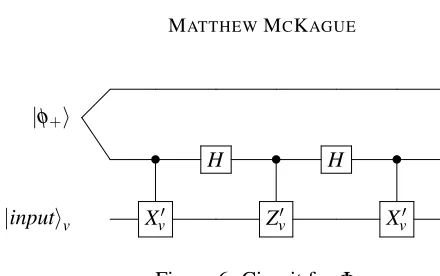
We will useΦvas defined inFigure 6. The circuit is modified from that used in [15,18] and earlier works, differing in the state of the ancilla. Whereas we use an entangled pair of qubits|φ+i, previous
works used|0i. We also add an initial CTRL-X gate which was not needed when the initial state was
|0i. WhenXv0andZv0 are the PauliX andZgates the circuit is clearly a SWAP gate. The idea is to swap a qubit embedded in the input wire with an explicit qubit in a new register.
As we shall see, the use of a maximally entangled pair of qubits in the ancilla wires allows for a tighter robustness analysis than is possible with the earlier version of the circuit. The reason is that the previous isometry used in [15] was very sensitive to error in the amplitude of|0. . .0i, but less so for other amplitudes. This is because|junkiis|ψ0iprojected down to the subspace corresponding to|0. . .0i. In
the new isometry|junkiis no longer projected down from|ψ0i, and the sensitivity to error is spread out
|φ+i
• H • H •
|inputiv Xv0 Zv0 Xv0
Figure 6: Circuit forΦv.
Proof. The structure of the proof is a sequence of chained inequalities between statesψj
andψj+1
for j=1. . .4 defined below. We then use the triangle inequality to find the total distance.|ψ1iis the state
immediately afterΦis applied.|ψ2i,|ψ3iand|ψ4iare the states after three successive applications of
Corollary 3.3. Finally,|ψ5iis the state after an application ofLemma 3.4. |ψ5iis then factored to give
|junkiand the ideal state|Gi.
We define the states|ψ1ithrough to|ψ5i:
|ψ1i:=Φ X0qZ0pψ0
=√1
23n
∑
s,t,u(−1)t·(s⊕u)X0uZ0tX0s⊕qZ0pψ0
|sui,
|ψ2i:=
1
√
23n
∑
s,t,u(−1)t·(s⊕u)(−1)p·(s⊕q)X0uZ0t⊕pX0s⊕qψ0
|sui,
|ψ3i:=
1
√
23n
∑
s,t,u(−1)t·(q⊕u)X0u⊕s⊕qZ0t⊕pψ0|sui,
|ψ4i:=
1
√
23n
∑
s,t,u(−1)t·s(−1)p·(u⊕s⊕q)Z0t⊕pX0u⊕s⊕qψ0|sui,
|ψ5i:=
1
√
23n
∑
s,t,u(−1)t·s(−1)p·u(−1)12(u⊕s)·A(u⊕s)Z0t⊕A(u⊕s)ψ0|si|u⊕qi
=|junkiXqZp|Gi.
Step 1: First we derive |ψ1i. LetΦ=Nv∈VΦv, and|ψ1i=Φ(X0qZ0p|ψ0i)to be the state after the
isometryΦis applied. Before the circuit is applied the state is
X0qZ0pψ0|φ+i⊗n=
1
√
2n
∑
sX0qZ0pψ0|ssi. (3.19)
Applying the first CTRL-X0gate yields 1
√
2n
∑
sX0sX0qZ0pψ0
|ssi. (3.20)
Next we multiply by the Hadamard gates and applyLemma 2.10to obtain
1
√
22n
∑
s,tThe CTRL-Z0gate produces
1
√
22n
∑
s,t(−1)t·sZ0tX0s⊕qZ0pψ0
|sti (3.22)
then another round of Hadamard and CTRL-X0gates yields
|ψ1i=
1
√
23n
∑
s,t,u(−1)t·(s⊕u)X0uZ0tX0s⊕qZ0pψ0|sui (3.23)
wheres,t,u∈ {0,1}n.
Step 2: In the ideal case,|ψ2iis obtained from|ψ1iby anti-commutingZ0pandX0s⊕q. Here we will
estimate|||ψ1i − |ψ2i||by usingCorollary 3.3. From the definition of the 2-norm,
|||ψ1i − |ψ2i||=
p
|||ψ1i||+|||ψ2i|| −2Rehψ1|ψ2i. (3.24)
We know that|||ψ1i||=1 because it was formed byΦapplied to a norm-1 state. For|||ψ2i||we have
hψ2|ψ2i=
1 23n
∑
s,s0 t,t0 u,u0
(−1)t·(s⊕u)(−1)t0·(s0⊕u0)(−1)p·(s⊕s0)ψ0X0s⊕qZ0t⊕pX0uX0u
0
Z0t0⊕pX0s0⊕qψ0 su|s0u0
. (3.25)
Thehsu|s0u0ifactor implies thatu0=uands0=sfor all non-zero terms so
hψ2|ψ2i=
1 23n
∑
s,t,t0u
(−1)(t⊕t0)·(s⊕u)ψ0X0s⊕qZ0t⊕pX0uX0uZ0t
0⊕ pX0s⊕q
ψ0. (3.26)
TheX0uoperators square to the identity, and subsequently so do theZ0ps. 1
23n
∑
s,t,t0u(−1)(t⊕t0)·(s⊕u)ψ0X0s⊕qZ0t⊕t
0
X0s⊕qψ0
. (3.27)
We then make a change of variablet07→t0⊕tand break(−1)t·(s⊕u)into(−1)t·s(−1)t·u. The summand no longer depends ont0 so we can omit it from the summation, multiplying by 2ninstead. We also bring the summation overuinside, forming an inner sum
1 22n
∑
s,t
(−1)t·s
∑
u(−1)t·u
ψ0X0s⊕qZ0tX0s⊕q ψ0
. (3.28)
Lemma 2.8says that the inner sum is 0 except whent=0, so we can drop theZ0ts and the summation
overt. Alsot·s=0. Then theX0s⊕qs then square to the identity. We are left with
|||ψ2i||=
1 2n
∑
s
Now we estimatehψ1|ψ2i:
hψ1|ψ2i=
1 23n
∑
s,s0 t,t0 u,u0
(−1)t·(s⊕u)(−1)t0·(s0⊕u0)(−1)p·(s0⊕q)
ψ0Z0pX0q⊕sZ0tX0uX0u
0
Z0t0⊕pX0s0⊕qψ0 su|s0u0. (3.30)
From thehsu|s0u0iterm, we see thats=s0 andu=u0 in all non-zero terms. This allows us to cancel
X0uX0u0 and remove theu0ands0variables. We also pull the sum overuin as an inner sum:
hψ1|ψ2i=
1 23n
∑
s,t,t0
∑
u(−1)(t⊕t0)·u
(−1)(t⊕t0)·s(−1)p·(s⊕q)
ψ0Z0pX0q⊕sZ0t⊕t
0
Z0pX0s⊕qψ0. (3.31)
Next we useLemma 2.8to see that the inner sum is zero except whent⊕t0=0. The terms(−1)(t⊕t0)·s)
andZ0t⊕t0 then become 1 and the identity, leaving the summand independent oftandt0. We remove them from the sum, multiplying by 2ninstead. Finally, we make the change of variables7→s⊕qto get
hψ1|ψ2i=
1 2n
∑
s
(−1)p·sψ0Z0pX0sZ0pX0s
ψ0. (3.32)
Next setεp,s= (−1)p·shψ0|Z0pX0sZ0pX0s|ψ0i − hψ0|Z0pX0sX0sZ0p|ψ0i, with the second term becoming just hψ0|ψ0i=1, so that the above becomes
hψ1|ψ2i=
1 2n
∑
s
(1+εp,s) =1+ 1 2n
∑
s
εp,s. (3.33)
Corollary 3.3and the third part ofLemma 2.7give|εp,s| ≤4(p·s)
√
2ε and the triangle inequality then gives us
|hψ1|ψ2i −1| ≤ 1
2n
∑
s4(p·s)
√
2ε. (3.34)
Lemma 2.9tells us how to deal with the sum overs, and we write
|hψ1|ψ2i −1| ≤2(p·p)
√
2ε (3.35)
and plugging this back into the definition of the 2-norm gives
|||ψ1i − |ψ2i|| ≤
q
4(p·p)√2ε. (3.36)
Step 3:Now let us look at|ψ2iand|ψ3i: |ψ2i:=
1
√
23n
∑
s,t,u(−1)t·(s⊕u)(−1)p·(s⊕q)X0uZ0t⊕pX0s⊕qψ0|sui,
|ψ3i:=
1
√
23n
∑
s,t,u|ψ3iis obtained from|ψ2iby moving theZ0s to the right, picking up a phase from the operators that
anti-commute. Following a argument similar to Step 2, we find
|||ψ2i − |ψ3i|| ≤
q
2n √
2ε. (3.37)
Step 4:Here is|ψ4ionce again: |ψ4i=
1
√
23n
∑
s,t,u(−1)t·s(−1)p·(u⊕s⊕q)Z0t⊕pX0u⊕s⊕qψ0
|sui.
We can see that|ψ4ican be had from|ψ3iby movingZ0to the left past theX0s, again using an argument
similar to Step 2. We find
|||ψ3i − |ψ4i|| ≤
q
2n√2ε. (3.38)
Step 5:Now we make two changes of variable,t7→t⊕pandu7→u⊕qand to find that
|ψ4i=
1
√
23n
∑
s,t,u(−1)t·s(−1)p·uZ0tX0u⊕sψ0
|si|u⊕qi. (3.39)
We will replace theX0s withZ0s usingLemma 3.4to obtain|ψ5i, which we recall to be |ψ5i=
1
√
23n
∑
s,t,u(−1)t·s(−1)p·u(−1)12(u⊕s)·A(u⊕s)Z0t⊕A(u⊕s)ψ0|si|u⊕qi.
Let us now calculate|||ψ4i − |ψ5i||. Again we proceed by way of the definition of||·||and the inner
product. First, we find|||ψ5i||=1 following an argument similar to that for|||ψ2i||in Step 2. Next we
estimatehψ4|ψ5i:
hψ4|ψ5i=
1 23n
∑
s,s0 t,t0 u,u0
(−1)t·s(−1)t0·s0(−1)p·(u⊕u0)(−1)12(u
0⊕s0)·A(u0⊕s0)
ψ0X0u⊕sZ0tZ0t
0⊕A(u0⊕s0)
ψ0 s,u⊕q|s0,u0⊕q.
(3.40)
For all non-zero terms we haves=s0 andu=u0. Re-indexing by s7→s⊕uwe find that the above is equal to
1 23n
∑
s,t,t0
∑
u(−1)(t⊕t0)·u
(−1)(t⊕t0)·s(−1)21s·Asψ0X0sZ0t⊕t
0⊕As
ψ0 (3.41)
where we have pulled all the terms dependent onuinto the inner sum. Lemma 2.8says that this inner sum is zero except wheret⊕t0=0 when it is 2n. Substituting these in, the above becomes
1 2n
∑
s
Now let us bound the inner product:
|1− hψ4|ψ5i|=
1− 1
2n
∑
s(−1)12s·Asψ0X0sZ0Asψ0
(3.43) ≤ 1
2n
∑
s
1−(−1)
1
2s·Asψ0X0sZ0Asψ0
(3.44) ≤ √ 2ε
2n
∑
s2(s·As) + (s·s) (3.45)
≤ |E|+n
2
√
2ε. (3.46)
To obtain the second line above we have used the triangle inequality. The third line comes from taking
Lemma 3.4, multiplying on the left byhX0s|and applyingLemma 2.7. We then useLemma 2.9to obtain
the last line. Finally we find
|||ψ4i − |ψ5i|| ≤
q
(|E|+n)
√
2ε. (3.47)
Adding all the bounds using the triangle inequality we obtain
|||ψ1i − |ψ5i|| ≤
2√p·p+2
√
2n+p|E|+n
(2ε)
1
4. (3.48)
Step 6: We now have an estimate for the distance between|ψ1iand|ψ5i. The final step is to show that |ψ5ifactors so that we can define|junki.
In|ψ5i, changing variablet7→t⊕A(u⊕s)we get |ψ5i=
1
√
23n
∑
s,t,u(−1)t·s(−1)p·u(−1)s·A(u⊕s)(−1)12(u⊕s)·A(u⊕s)Z0tψ0|si|u⊕qi (3.49) and applyingLemma 2.11cleans this up to
1
√
23n
∑
s,t,u(−1)t·s(−1)p·u(−1)12s·As(−1)12u·AuZ0tψ0|si|u⊕qi (3.50) after which the state factors as follows:
|ψ5i=
1
√
23n
∑
s,t(−1)t·s(−1)12s·Asψ0|si
∑
u(−1)p·u(−1)12u·Au|u⊕qi
= 1
2n
∑
s,t(−1)t·s(−1)21s·AsZ0tψ0|si
!
XqZp|Gi. (3.51)
Setting
|junki:= 1
2n
∑
s,t(−1)t·s(−1)12s·AsZ0tψ0|si (3.52) we can finally state
Φ X0qZ0p ψ0
− |junkiXqZp|Gi ≤
2√p·p+2
√
2n+p|E|+n
(2ε)
1
4 (3.53)
3.2 Error bounds for non-Pauli measurements
In order to achieve universal computation we need to have measurements other than justX andZ. It suffices to haveX-Zplane measurements. Let us define
Rv(θ) =cosθXv+sinθZv. (3.54) We use the symbolR0u(θ)to denote the±1 eigenvalue observable that the prover uses when queried with
the angleθ. We do not make any prior assumption on howR0u(θ)is related toXu0orZu0. Instead we will derive said relationship via the graph-state test and further measurements.
Lemma 3.5. Under the conditions ofTheorem 3.1, if we have measurements R0v(θ)and an edge(u,v)
such that
ψ0R0v(θ)
cosθZ0A1v+sinθXu0Z0A1u⊕1v
ψ0
≥1−ε (3.55)
then withΦand|junkiset to those inTheorem 3.1,
Φ(R0v(θ)
ψ0)− |junkiRv(θ)|ψi
≤
p
2(ε+2δ) (3.56)
whereδ is the bound inTheorem 3.1.
Proof. FromTheorem 3.1we obtainΦand|junkiso that
Φ(M0
ψ0)− |junkiM|ψi
≤δ (3.57)
forM0∈ {Z0A1v,X0
uZ0A1u⊕1v}in particular. From the stabilizer generatorsSuandSvwe find XuZA1u⊕1v|ψi=Zv|ψi and ZA1v|ψi=Xv|ψi,
hence linearity ofΦand the triangle inequality give
Φ
cosθZ0A1v+sinθXu0Z
0A1u⊕1v ψ0
− |junki(cosθXv+sinθZv)|ψi
≤(cosθ+sinθ)δ. (3.58)
Using cosθXv+sinθZv=Rv(θ)and cosθ+sinθ≤2 this becomes
Φ
cosθZ0A1v+sinθXu0Z
0A1u⊕1v ψ0
− |junkiRv(θ)|ψi
≤2δ. (3.59)
Now since||hψ0|Φ(R0v(θ))||∞=1, we have
Φ
ψ0R0v(θ)
Φ
cosθZ0A1v+sinθXu0Z
0A1u⊕1v ψ0
−Φ ψ0R0v(θ)
|junkiRv(θ)|ψi ≤2δ.
(3.60)
Φpreserves inner products, so this becomes
ψ0R0v(θ)
cosθZ0A1v+sinθXu0Z0A1u⊕1v
ψ0−Φ ψ0R0v(θ)
|junkiRv(θ)|ψi
≤2δ. (3.61)
Using the triangle inequality and (3.55) we find
The lemma says that if we can estimate the expected value for a certain operator we can bound the error onR0u(θ). Later inSection 3.4we will show how we can estimate said expected value.
3.3 Error bounds for measurement patterns
Our bounds inSection 3.1show that we can bound the error when applying a measurement of the formM1⊗ · · · ⊗Mn, which gives a single bit of output. However, for graph state computation we need something much more substantial since we will need to measure the subsystems in a sequence, with each basis chosen as a function of the previous outcomes. In fact we will prove something even stronger than this.
We will consider a more general situation where instead of trusted classical computation and classical interaction, we have some trusted quantum computation and quantum interaction with the provers. The provers allow the basis to be chosen quantumly and they similarly return the result coherently. We can model this by specifying that, when queried with a quantum register, prover japplies
Vj0=
mj
∑
k=0|kihk| ⊗M0j,k (3.63)
whereM0j,kcorresponds to the observable that prover juses when queried with inputk∈ {0. . .mj}. The prover then passes the control register back to the verifier and the result of the query is stored as a±1 phase. We will require that the prover’s actions are all of this form, although they are free to choose the
M0j,k as they like. As well, the ideal operatorVj has this form, using observablesMj,k.
Assuming5M0j,0=Iwe can retrieve the outcome for measurementM0j,kby preparing the state 1
√
2(|0i+|ki)
and observing the relative phase change in the prover’s response. Hence this model includes the original classical behavior as a particular case.
A general circuit for the verifier-prover interaction in this stronger model is given inFigure 7. The verifier first applies some unitaryU0to prepare its initial state, and then performs the first query to prover
1,V10. The verifier then applies some unitaryU1to its internal state and performs the second query to prover 2,V20, and so on. The combined operation isUnVn0. . .U1V10U0. We require that eachVj0is applied at most once and for convenience we suppose that they are numbered in the order in which they are applied. In this circuit we have always used the same the control wire, which is a q-dit with dimension equal to the maximummj+1. This is not a limitation since we can always use the same control wire by incorporating swaps into theU’s if necessary.
LetW00=U0, andWj0=UjVj0Wj0−1for j≥1. That is,Wj0represents running the circuit until the point afterUjhas been applied. Similarly, letWj =UjVjWj−1be the ideal circuit where we substitute in the
idealVj(constructed from the idealMj,k).
5Our current self-test doesn’t test whether the identity is performed correctly, but this should always give the outcome 1 so
U0 U1 U2 Trusted . . . • • •
V10
Untrusted
V20 . . . V30
.. .
Figure 7: Semi-trusted circuit incorporating untrusted measurements by the provers,Vj0.
Lemma 3.6. Let|ψi,|ψ0i,|junki, andΦ=Φ1⊗ · · · ⊗Φnbe given along with M0j,kand Mj,k(k=0. . .m and M0j,0=I) such that
Φ M0j,k
ψ0
− |junkiMj,k|ψi
≤δ. (3.64)
Further, let some|φiand Uj be given where|φicontains a register of dimension at least m+1and Uj acts only on the|φiregisters, and let, Vj, Vj0, Wj and Wj0be defined as above. Then
Φ(Wn0
ψ0|φi)− |junkiWn|ψi|φi
≤(2nm+1)δ. (3.65)
The intuition is that eachVj0 is the sum of operators |kihk| ⊗M0j,k, each of which is close to the corresponding ideal operator. We can then use the triangle inequality to say thatVj0as a whole is close to its ideal counterpart. Inducting over the depth of the circuit gives the desired result.
Proof. The proof proceeds by induction. For the casen=0 we have not yet applied any untrusted gates and the conclusion is true by taking inequality (3.64) withk=0 and multiplying by the trusted gateU0.
Now let us suppose that (3.65) holds forn−1. We start by using the bound (3.64) with(j,k) = (1,0)
to get Φ ψ0
− |junki|ψi
≤δ. (3.66)
For eachk6=0 we multiply on both sides byΦn(Mn,k0 )to obtain inequalities
Φn(Mn,k0 )|junki|ψi −Φn(Mn,k0 )Φ(
ψ0)
≤δ. (3.67)
ByLemma 2.6,Φn(Mn,k0 )Φ(|ψ0i) =Φ(Mn,k0 |ψ0i), so the state on the right above is close to|junkiMn,k|ψi
by (3.64) with(j,k) = (n,k). Using the triangle inequality we find
Φn(Mn,k0 )|junki|ψi − |junkiMn,k|ψi
≤2δ. (3.68)
We introduce the register|φi and apply the ideal unitaryWn−1 to both sides in the above estimation
with thenth subsystem of|ψi). Then sinceWn−1operates only on the trusted system and the firstn−1
subsystems of|ψi, it commutes withΦn(Mn,k0 )andMn,k so
Φn(Mn,k0 )|junkiWn−1|ψi|φi − |junkiMn,kWn−1|ψi|φi
≤2δ. (3.69)
Now we apply the projection|kihk|(used in the expression forVn0) to both sides, again without increasing the distance. Hence
|kihk| ⊗Φn(Mn,k0 )Wn−1|junki|ψi − |junki|kihk| ⊗Mn,kWn−1|ψi
≤2δ. (3.70)
Summing over allkusing triangle inequality, we apply the definitions ofVjandVj0 to arrive at
Φ(Vn0)|junkiWn−1|ψi|φi − |junkiVnWn−1|ψi|φi
≤2mδ. (3.71)
Note that it is 2mδ and not 2(m+1)δ since the casek=0 has no error by assumption. The state on
the right above is almost what we want. Now we invoke the induction hypothesis (3.65) withn−1 and multiply through byΦ(Vn0)to get
Φ(Vn0Wn0−1 ψ0
|φi)−Φ(Vn0)|junkiWn−1|ψi|φi
≤2m(n−1)δ (3.72)
and applying the triangle inequality to the above two estimates we get
Φ(Vn0Wn0−1
ψ0|φi)− |junkiVnWn−1|ψi|φi
≤2mnδ. (3.73)
Multiplying by the trusted gateUn(which commutes withΦ) finishes the proof.
For our purposes we do not need the full strength of the lemma. We need only know that adaptive measurements give correct outcomes, which we prove in the following corollary.
Corollary 3.7. Let|ψi,|ψ0i,|junki, andΦ=Φ1⊗· · ·⊗Φnbe given along with M0j,kand Mj,k(k=0. . .m and M0j,0=I) such that
Φ M0j,k
ψ0− |junkiMj,k|ψi
≤δ. (3.74)
Then for any adaptive measurement made using the M0s, the probability of a particular outcome differs from the ideal case by at most2(2nm+1)δ.
Proof. We can represent an adaptive measurement as a circuitWnas inLemma 3.6. Hence
Φ(Wn0
ψ0
|φi)− |junkiWn|ψi|φi
≤(2nm+1)δ. (3.75)
To obtain the classical outcome we perform some measurement on one of the trusted subsystems. Without loss of generality this can be a projective measurement, so letΠx be the projector for outcomex, which acts non-trivially only on the trusted subsystem. The probability of outcomexis then
ψ0hφ|Wn†0ΠxWn0 ψ0
Now to estimate this probability we use (3.75) above in two different ways. First, multiplying on the left byΦ(hψ0|hφ|Wn†0)Πxwe get
Φ(
ψ0hφ|Wn†0)ΠxΦ(Wn0
ψ0
|φi)−Φ(ψ0hφ|Wn†0)Πx|junkiWn|ψi|φi≤(2nm+1)δ. (3.77)
Second, multiplying (3.75) on the left byhjunk|hψ|hφ|Wn†Πx and then taking the adjoint of the resulting expression we obtain
Φ(
ψ0hφ|Wn†0)Πx|junkiWn|ψi|φi − hψ|hφ|Wn†ΠxWn|ψi|φi
≤(2nm+1)δ. (3.78)
Adding these together using the triangle inequality and invoking the fact thatΦpreserves inner products we find
ψ0hφ|Wn†0ΠxWn0 ψ0
|φi − hψ|hφ|Wn†ΠxWn|ψi|φi
≤2(2mn+1)δ. (3.79)
In other words, the probability of finding outcomexdiffers from the ideal case by at most 2(2mn+
1)δ.
3.4 A one-shot test
As stated, the self-testing results are not terribly useful to us. They require knowledge of the expected value of various operators in order to draw any conclusions. The obvious solution is to take some samples and estimate, but this would require either some independence assumptions or additional work with, for example, martingales as is done in [23]. Instead we will work with the contrapositive of the self-testing results: if the state and/or some measurements are far away from the ideal, then some measurable expected value will also be far away from the ideal. Although this is logically equivalent, instead of requiring lots of information about the various measurements, we instead are told that we just have to look for one measurement that is misbehaving.
As well, we are going to arrange our measurements in a particular way as a test for honesty. For example, the stabilizer measurements will always return 1 for honest provers, so if we perform this measurement and we get a 1 the provers pass the test. If result is -1 then they fail the test. As the expected value gets close to 1, the provers will pass with probability close to 1. If the expected value is far away from 1, the provers will fail the test with some probability.
Now with theR(θ)measurements we do not have the same situation, but we do have something just
as useful. We can build a compound test so that the ideal honest provers pass with some probability, and no other provers can pass with a higher probability. This is analogous to the CHSH test: the ideal quantum strategy passes with probability≈0.85, and no other strategy achieves any higher success rate. As well, cheating provers will pass the test with a probability that is bounded away from the quantum limit, and so we obtain a gap between the ideal and cheating strategies. The honest provers will fail the test some of the time, but this is no problem: we will later do some repetition so that the ideal provers will pass with an overall probability that can be made arbitrarily close to 1.
Now we give the construction for our one-shot test. Fix a graphG= (V,E)in which every vertex appears in a triangle and setn=|V|. LetT be a set of triangles that coversV, i. e., each vertex inV
appears in at least one triangle inT. The triangles will be specified by characteristic vectorsτ. Let
For a graph state computation we need only two different measurement angles per vertex,±θv. As well, the measurement angle θv+π can be simulated by measuring with angles θv and flipping the outcome. Hence there is no loss of generality by assuming that 0≤θv≤πso that cosθv≥0.
The test procedure is as follows:
Procedure 2(One-shot test for graph states and measurements).
1. Randomly select either “VERTEX” with probability |V|/NG, “TRIANGLE” with probability |T|/NG, or “RTHETA” with probability 2|V|/NG.
2. if “VERTEX,”
(a) Selectv∈RV.
(b) Query the provers with bases according toSV =XvZA1v. (c) Accept if the product of the replies is 1, otherwise reject.
3. if “TRIANGLE,”
(a) Selectτ∈RT.
(b) Query the provers with bases according toXτZAτ.
(c) Accept if the product of the replies is -1, otherwise reject.
4. if “RTHETA,”
(a) Chooset∈R{1,−1}andv∈RV and letube a vertex adjacent tov. (ucan be fixed ahead of time for eachv.)
(b) Choose eitherX with probability cosθv cosθv+|sinθv|
orZwith probability |sinθv| cosθv+|sinθv|
.
(c) ifX,
i. Query the provers withRv(tθv)vZA1v.
ii. Accept if the product of the replies is 1, otherwise reject.
(d) ifZ,
i. Query the provers withtRv(tθv)XuZA1u⊕1v.
ii. Accept if the product of the replies is 1, otherwise reject.
To clarify, if the basis for a prover isIthen we simply ignore that prover, and its “reply” is taken to be 1.
Lemma 3.8. Let n non-communicating quantum provers be given that each take one of four measurement bases, labeled X , Z and Rv(±θv) as inputs and measure joint state |ψ0i according to operators in {Xv0,Zv0,R0v(θv)}. ThenProcedure 2accepts with probability at most
ctest=
2|V|+|T|+∑vcosθ 1 v+|sinθv| NG
(honest case) (3.80)
and if there exist v and M∈ {Xv,Zv,Rv±θv)v}such
Φ M0
ψ0
− |junkiM|Gi
>δ (3.81)
thenProcedure 2accepts with probability at most
ctest−
1 2NG
δ2
22+25√n
4
(dishonest case). (3.82)
Proof. Honest case. First let us derive the maximum probability of passing the test. This is attained in the honest case. The “VERTEX” and “TRIANGLE” subtests can all be passed simultaneously with probability 1 in the honest case since the observables are all in the stabilizer group of the graph state.
Let us now consider the “RTHETA” subtests. First, we fix a vertexv. The queries to the provers in this subtest can be seen as one large random variable taking values±1 and having the expected value
1
2(cosθv+|sinθv|)
ψ0R0v(θv)
cosθvZ0A1v+sinθvXu0Z0A1u⊕1v
ψ0
+
ψ0R0v(−θv)
cosθvZ0A1v−sinθvXu0Z0A1u⊕1v
ψ0
. (3.83)
Note the similarity to the CHSH correlation, which is obtained forθv=π/4. The honest provers (withR0v(θv) =Rv(θv)) will attain an expected value of
1
2(cosθv+|sinθv|) .
To see this, we notice thatZA1v|ψi=Xv|ψiandXuZA1u⊕1v=Zv|ψi, which we obtain from the stabilizers
SvandSu, respectively. Applying the definition ofR(θ), the expected value becomes 1
2(cosθv+|sinθv|)
hψ| Rv(θv)2+Rv(−θv)2
|ψi= 1
cosθv+|sinθv|
(3.84)
sinceR2v(θv) =I.
Now we show that this is in fact the maximal quantum expected value. Using a standard technique introduced by Cirel’son [6], the maximum value is the same as
1
2(cosθv+|sinθv|)
max
|ψ1i,|ψ2i,|φ1i,|φ2i