http://theoryofcomputing.org
Removing Degeneracy May Require a Large
Dimension Increase
∗
Jiˇr´ı Matouˇsek
Petr ˇSkovroˇn
Received: March 12, 2007; published: September 26, 2007.
Abstract: Many geometric algorithms are formulated for input objects in general position;
sometimes this is for convenience and simplicity, and sometimes it is essential for the al-gorithm to work at all. For arbitrary inputs this requires removing degeneracies, which has usually been solved by relatively complicated and computationally demanding perturbation methods.
The result of this paper can be regarded as an indication that the problem of removing degeneracies has no simple “abstract” solution. We consider LP-type problems, a successful axiomatic framework for optimization problems capturing, e. g., linear programming and the smallest enclosing ball of a point set. For infinitely many integers D we construct a D-dimensional LP-type problem such that in order to remove degeneracies from it, we have to increase the dimension to at least(1+ε)D, whereε >0 is an absolute constant.
The proof consists of showing that certain posets cannot be covered by pairwise disjoint copies of Boolean algebras under some restrictions on their placement. To this end, we prove that certain systems of linear inequalities are unsolvable, which seems to require surprisingly precise calculations.
∗An extended abstract of this paper has appeared in Proceedings of European Conference on Combinatorics, Graph Theory
and Applications 2007 (Eurocomb), pp. 107–113.
ACM Classification: F.2.2
AMS Classification: 68U05, 06A07, 68R99
Key words and phrases: LP-type problem, degeneracy, general position, geometric computation,
par-tially ordered set
1
Introduction
Geometric computation and degeneracy. Many descriptions of algorithms in computational geom-etry or in geometric optimization, as well as numerous proofs in discrete geomgeom-etry, start with a sentence similar to “Let us assume that the given points are in general position.” General position may mean that no three among the points are collinear, or we may also require than no four are cocircular, etc., depending on the considered problem. Violations of general positions, such as three points on a line, are referred to as degeneracies.
Assuming the input to be nondegenerate (i. e., in general position) usually simplifies the description, analysis, and implementation of a geometric algorithm significantly. For many algorithms, this assump-tion can be avoided with some extra work and careful attenassump-tion to detail (a case study, arguing in favor of expending such extra work, is Burnikel et al. [4]). However, for some algorithms, the nondegeneracy as-sumption is not only a convenient simplification, but rather an essential condition for correctness and/or for running time analysis, which seems difficult to circumvent—we will mention an example below.
General methods have been developed for removing degeneracies in geometric algorithms, based on
infinitesimal perturbations of the input (Edelsbrunner and M¨ucke [8], Yap [22], Emiris and Canny [9]). Roughly speaking, the coordinates of each input object are changed by a suitable function of a real parameterε >0, and the considered algorithm is executed with these new input objects, treatingε as a formal quantity, smaller than any concrete nonzero real number occurring in the algorithm. These approaches can actually be implemented, but they have several drawbacks: They slow down the compu-tations significantly (typically by a large constant factor, but sometimes even much more), they increase space requirements, and sometimes it may be difficult or impossible to reconstruct the correct result for the original input from the result for the perturbed input—see [4] for a discussion.
Removing degeneracies means “breaking ties” in some sense. Of course, the ties cannot be broken arbitrarily, since geometric algorithms almost always depend on some kind of global consistency of the input. Still, one might hope for some simpler, perhaps combinatorial, way of removing degeneracies.
To illustrate what we have in mind, let us recall that the famous simplex method of linear program-ming may also suffer from degeneracy—namely, for many pivoting rules the simplex method may get into an infinite loop (to cycle) for certain highly degenerate inputs. (However, unlike degeneracy in the geometric computations mentioned above, cycling of the simplex method is not an issue in prac-tice.) There are two well-known pivot rules that provably avoid cycling: the lexicographic rule, which is conceptually an infinitesimal perturbation, and Bland’s rule, which is a combinatorial rule working solely with indices of variables and constraints, as opposed to geometric properties of the input. So our question is, whether there is something like a general “Bland’s rule” that would allow one to avoid degeneracies in (some interesting classes of) geometric algorithms.
The present work can be regarded as an indication that a simple, general, and efficient combinatorial method is unlikely to exist.
problems, as well as e. g. [21,12,10,18] for the investigation of other, related frameworks.
Once it is shown that a particular optimization problem is an LP-type problem and certain algo-rithmic primitives are implemented for it, several efficient algorithms are immediately at disposal: the Sharir–Welzl algorithm, two other randomized optimization algorithms due to Clarkson [7] (see [13,6] for a discussion of how it fits the LP-type framework), a deterministic version of it [6], and an algorithm for computing the minimum solution that violates at most k of the given n constraints [16] (this is the promised example of an algorithm where nondegeneracy appears crucial).
An LP-type problem is given by a finite set H of constraints and a value w(G)∈Rfor every subset
G⊆H. Intuitively, w(G)is the minimum value of a solution that satisfies all constraints in G. As our running example, we will use the problem of computing the smallest disk containing a given planar point set. Here H is a finite point set inR2and w(G)is the radius of the smallest circular disk that encloses
all points of G. The general definition is as follows:
Definition 1.1. An LP-type problem is a pair(H,w), where H is a finite set and w : 2H→Ris a mapping satisfying the following two conditions:1
Monotonicity: For all F ⊆G⊆H we have w(F)≤w(G). Locality: For all F ⊆G⊆H and all h∈H,
if w(F) =w(G) =w(F∪ {h})then w(G∪ {h}) =w(G).
For the smallest enclosing disk problem, monotonicity is obvious, while verifying locality requires the nontrivial but well known geometric result that the smallest enclosing disk is unique for every set.
The most important parameter of an LP-type problem, essentially controlling the behavior of algo-rithms dealing with the given problem, is the combinatorial dimension.
Definition 1.2. Let(H,w)be an LP-type problem and let G⊆H. A basis of G is any inclusion-minimal
subset B⊆G with w(B) =w(G). A set B⊆H is called a basis in(H,w)if it is a basis of some G⊆H.
The combinatorial dimension of(H,w)is the maximum cardinality of a basis.
If(H,w)is a smallest enclosing disk problem, then the combinatorial dimension is at most 3 (since for every point set G in the plane there is a subset B of at most 3 points of G such that G and B have the same smallest enclosing disk). Similarly, a higher-dimensional version, the smallest enclosing ball problem of a point set inRd, has combinatorial dimension at most d+1.
Degeneracy in LP-type problems. What should be considered a degeneracy in the smallest enclos-ing disk problem? A reasonable answer is a subproblem with an “overdetermined” solution, which means a set G whose minimum enclosing disk is determined by two distinct inclusion-minimal subsets
B1,B2⊆G. For example, B1 and B2 can be two different diametrical pairs determining the same disk. Nondegeneracy for an arbitrary LP-type problem can be defined in a similar way [16].
1Actually, the usual definition of an LP-type problem is more general: the mapping w can also attain a special value−∞,
which is considered smaller than all real numbers, and for which the locality axiom is not required. Moreover, instead ofR,
a b c d
Figure 1: A degenerate LP-type problem where removing degeneracy increases dimension.
Definition 1.3. We call an LP-type problem(H,w)nondegenerate if w(B1)6=w(B2)for any two distinct bases B1,B2.
Consequently, in a nondegenerate LP-type problem, every G⊆H has exactly one basis.2
For removing degeneracies, we want to break the ties w(B1) =w(B2) by slightly modifying the values of w, while retaining all strict inequalities among the original values:
Definition 1.4. An LP-type problem(H,w0)is a refinement of an LP-type problem(H,w)on the same set of constraints if for all F,G⊆H with w(F)<w(G)we have w0(F)<w0(G).
We thus formalize “removing degeneracies” of an LP-type problem(H,w)as the question of finding a nondegenerate refinement of(H,w).
At first sight it might seem that in order to produce a nondegenerate refinement, it should suffice to impose some suitable linear order on every group of bases sharing the same value of w—perhaps one could even take an arbitrary ordering.
However, some thought reveals that things are not that simple. As was observed in [16], sometimes we also have to create new bases, and even larger ones than those present in(H,w). Namely, consider the smallest enclosing disk problem with H={a,b,c,d}forming the vertices of a square (Figure 1). The set H has two bases B1={a,c}and B2={b,d}, and the combinatorial dimension of the problem is 2. We will refer to this particular 2-dimensional LP-type problem as the square example and denote it by(Hsq,wsq). It is easily checked (we will do so inSection 2) that any nondegenerate refinement has dimension at least 3. Hence removing degeneracies necessarily increases the dimension by 2.
In a preliminary report [20] containing some of the results of the present paper, an LP-type problem was presented where removing degeneracy forces dimension increase by 2. Here we exhibit LP-type problems where the required increase is arbitrarily large.
Theorem 1.5. There exists a positive constantε >0 such that for infinitely many values of D, there
is an LP-type problem of combinatorial dimension D, for which every nondegenerate refinement has combinatorial dimension at least(1+ε)D.
The example of an LP-type problem as in the theorem is obtained by an “iterated join” of the square example. We also show that an essentially equivalent example can be represented as a linear program in the usual sense (a highly degenerate linear program).
2Another, seemingly weaker, notion of nondegeneracy naturally coming to mind is to require that every G⊆H has a unique
The result can also be understood as telling us that for degenerate LP-type problems, the combina-torial dimension doesn’t convey a full “dimensionality” information about the problem. An alternative dimension parameter might be the smallest possible dimension of a nondegenerate refinement; however, this appears quite hard to determine.
The main open question is, can the smallest possible dimension of a nondegenerate refinement be bounded by some function of the dimension of the original degenerate LP-type problem? In particular, does every 2-dimensional LP-type problem have a nondegenerate refinement of dimension bounded by a universal constant? We suspect that it is not the case, but it seems that the methods of the present paper are not sufficient to yield such a result. The structure of 2-dimensional LP-type problems, say, appears both quite restricted and hard to describe, and at present we have no candidate for an LP-type problem where removing degeneracies might require increasing the dimension by more than a small constant factor.
2
Structure of nondegenerate LP-type problems
Let(H,w) be an LP-type problem. We consider the partially ordered set (poset)(2H,⊆), a Boolean algebra. For every x∈R, we define the set systemPx={G⊆H : w(G) =x}. ThePxfor all x∈Rform
a partition of 2H. Monotonicity implies thatPx has no “holes”: If F⊂M⊂G and x=w(F) =w(G), then w(M) =x as well. The following lemma shows that for nondegenerate LP-type problems, eachPx is actually a copy of a Boolean algebra.
Lemma 2.1 (Cube lemma). Let(H,w) be a nondegenerate LP-type problem. For every x∈Rwith
Px6= /0 there exist two (uniquely determined) sets B,C⊆H such thatPx={F ⊆H : B⊆F⊆C}. The set B is the basis of all F∈Px.
We call the set{F⊆H : B⊆F⊆C}a cube, we use the notation[B,C]for it, we call B the bottom
vertex and C the top vertex of the cube[B,C], and|C\B|is the dimension of the cube.
Proof. We choose G∈Pxarbitrarily, we let B be the basis of G, and we set C=nh∈H : w(B) =w(B∪ {h})o .
We claim that this choice of B and C satisfies the desired conditions. First we prove that w(B) =w(C). Letting C\B={c1, . . . ,cm}, we check by induction that w(B) =w(B∪ {c1, . . . ,ci}), i=0,1, . . . ,m. Indeed, the induction step from i to i+1 follows immediately from the locality axiom with F=B, G= B∪ {c1, . . . ,ci}, and h=ci+1. Now when we have w(B) =w(C), monotonicity implies that[B,C]⊆Px. Now let us assume w(F) =w(B)for some F⊆H. Let B0be a basis of F; we have w(B0) =w(F) = w(B), and thus B=B0 by nondegeneracy. In particular, B⊆F. For every f ∈F we have w(B)≤ w(B∪ {f})≤w(F) =w(B), so w(B) =w(B∪ {f}), and hence f ∈C; thus F⊆C. Since F was an
arbitrary set inPxand we have obtained B⊆F⊆C, we conclude withPx⊆[B,C].
abcd
bcd abd acd
abc
bd ac
Figure 2: The posetPwsq(Hsq)for the square example.
To see how this lemma can be used, let us check the claim made in the introduction: every nonde-generate refinement of the square example(Hsq,wsq)has dimension at least 3. The posetPwsq(Hsq)of all subsets of Hsqwith the same smallest enclosing circle as that of Hsqconsists of all subsets of{a,b,c,d} containing{a,c}or{b,d}; seeFigure 2.
In any nondegenerate refinement,Pwsq(Hsq)has to be expressed as a disjoint union of cubes, and if the dimension of the refinement were 2, all of these cubes would have to have a 2-element set as the bottom vertex. In order to cover{a,b,c,d}, we have to use a 2-dimensional cube, say[{a,c},{a,b,c,d}]. To cover the remaining sets{b,d},{a,b,d}, and{b,c,d}by disjoint cubes, we must use at least one of the 0-dimensional (single-vertex) cubes[{a,b,d},{a,b,d}]or[{b,c,d},{b,c,d}]with a 3-element bottom vertex. Therefore a combinatorial dimension of any nondegenerate refinement of(Hsq,wsq)is at least 3.
3
The construction
We begin by defining a binary operation on LP-type problems.
Definition 3.1. Let(H1,w1) and(H2,w2) be LP-type problems, and assume H1∩H2= /0. We define a new LP-type problem, denoted by(H,w) = (H1,w1)∗(H2,w2) and called the join of(H1,w1) and (H2,w2): H :=H1∪H2and w(G):=w1(G∩H1) +w2(G∩H2)for all G⊆H.
Lemma 3.2. The join(H,w) = (H1,w1)∗(H2,w2) is indeed an LP-type problem, and dim(H,w) = dim(H1,w1) +dim(H2,w2).
Proof. First we observe that if F⊆G and w(F) =w(G), then wi(F∩Hi) =wi(G∩Hi), i=1,2. Indeed, since F∩Hi⊆G∩Hi, we have wi(F∩Hi)≤wi(G∩Hi), and to get equality of the sum, equality must hold in both components.
Now we verify the axioms for(H,w). Monotonicity is obvious, and for locality, let F⊆G⊆H and h∈H satisfy w(F) =w(G) =w(F∪ {h}). Supposing h∈H1, we have w1(F∩H1) =w1(G∩H1) = w1((F∩H1)∪ {h}) by the observation above, and locality in (H1,w1) yields w1((G∩H1)∪ {h}) = w1(G∩H1). Then
Now we check dim(H,w)≥dim(H1,w1) +dim(H2,w2). Let Bi be a basis in(Hi,wi) witnessing dim(Hi,wi). It suffices to check that B=B1∪B2 is a basis in(H,w); that is, w(A)<w(B)for every proper subset of B. Letting Ai=A∩Hi, we have Ai⊆Biwith at least one of the inclusions proper, say A1⊂B1. Since B1is a basis, we have w1(A1)<w1(B1)and w(A)<w(B)follows.
For the opposite inequality dim(H,w)≤dim(H1,w1) +dim(H2,w2), we choose a basis B in(H,w) with|B|=dim(H,w)and set Bi=B∩Hi. It suffices to check that Biis a basis in(Hi,wi). Let us consider a proper subset A1⊂B1; then
w1(B1) +w2(B2) =w(B1∪B2)>w(A1∪B2) =w1(A1) +w2(B2) , and we get w1(A1)<w1(B1)as needed. The lemma is proved.
The example. For the proof ofTheorem 1.5we define, for a natural number m, an LP-type problem
Lm as the m-fold join of the square example (Hsq,wsq). More formally, we choose distinct elements a1, . . . ,am, b1, . . . ,bm, c1, . . . ,cm, d1, . . . ,dm, we let Hi ={ai,bi,ci,di}, and we let wi: Hi →R be a
“copy” of the value function wsqfrom the square example, defined on Hi. We let
Lm= (H,w) = (H1,w1)∗ · · · ∗(Hm,wm)
(we note that the operation of join is clearly associative). We have|H|=4m and by the above lemma,
Lmis an LP-type problem of combinatorial dimension D=2m. It is easy to check that by taking a join of m suitable nondegenerate refinements of the square example we obtain a nondegenerate refinement of(H,w)of combinatorial dimension 3m.
We want to bound from below the dimension of any nondegenerate refinement ofLm. Similar to the warm-up argument for(Hsq,wsq), any nondegenerate refinementL0= (H,w0)ofLm of dimension D0 yields a covering of the posetPw(H)={G⊆H : w(G) =w(H)} by disjoint cubes[Bj,Cj], where each bottom vertex Bjsatisfies|Bj| ≤D0. We will deal with this combinatorial problem in the next two sections.
4 5 6 7 8
Figure 3: The posetPw(H)for m=2. The numbers in the right indicate sizes of the corresponding sets.
4 5 6 7 8
4
Setting up a linear system
The basic strategy for the proof ofTheorem 1.5is simple. LetLm= (H,w)be the example constructed above and let us suppose that the poset P:=Pw(H)⊂2H can be covered by disjoint cubes [Bj,Cj] with |Bj| ≤D0. Since dim(H,w) =D=2m and all bases of (H,w) have exactly this size, we have 2m≤ |Bj| ≤ |Cj| ≤ |H|=4m for all j. Let xd,k denote the number of cubes with|Bj|=2m+d and |Cj|=2m+k, d≤∆:=D0−2m, d≤k≤2m. A cube[Bj,Cj]with|Bj|=2m+d and|Cj|=2m+k contains sets of cardinality 2m+`, d≤`≤k, and the number of sets of this cardinality in[Bj,Cj]equals
k−d
`−d
(this formula is actually valid for all`if we adopt the convention that ab=0 for b<0 or b>a).
If we let
F(m, `) =|{G∈P:|G|=2m+`}| , we get that the xk,dhave to satisfy the following system of linear equations:
∆
∑
d=0 2m
∑
k=max(d,`)
k−d
`−d
xd,k=F(m, `) , `=0,1, . . . ,2m . (4.1)
We are going to prove that with ∆=dεDe, where ε is a sufficiently small positive constant, this system of equations for variables xk,d has no nonnegative real solution, provided that m is sufficiently large.
To see that an approach based on counting sets of individual cardinalities may help us to prove nonexistence of the covering ofP, note that already the proof in the end ofSection 2may be rephrased in terms of counting. In the poset inFigure 2, the vector of numbers of sets of cardinality 2, 3, and 4 is(2,4,1). However, this vector cannot be obtained as a nonnegative linear combination of vectors
(1,0,0),(1,1,0), and(1,2,1), which give numbers of sets of the respective cardinalities in cubes with the allowed cardinality of the bottom vertex.
First we evaluate F(m, `).
Lemma 4.1. We have
F(m, `) =
∑
s
m
s, `−2s,m−`+s
2m+`−3s ,
with the sum being over all s with 0≤2s≤`and s≥`−m (here k n
1,k2,k3
=k n!
1!k2!k3! is a multinomial
coefficient, k1+k2+k3=n).
Proof. First we observe, reasoning as in the proof ofLemma 3.2, that a set B⊆H is a basis of H in Lmif and only if each Bi=B∩Hi is a basis of Hiin(Hi,wi). Hence the bases of H are the sets B with B∩Hi={ai,ci}or B∩Hi={bi,di}for all i=1,2, . . . ,m. A set G⊆H is inPiff it contains at least one of these bases; i. e., if it contains at least one of the pairs{ai,ci},{bi,di}for all i.
For G∈Pof cardinality 2m+` let sr=|{i∈ {1,2, . . . ,m}:|G∩Hi|=r}|, r=2,3,4. We have s2+s3+s4=m and 2s2+3s3+4s4=|G|=2m+`. Calculation shows that s2=m−`+s4and s3=
`−2s4.
For counting the number of possible ways of choosing G, we first fix s=s4. Then s2and s3are fixed as well, and there are s m
2,s3,s4
there are two possibilities for G∩Hi, for|G∩Hi|=3 we have 4 possibilities, and for|G∩Hi|there is just one possibility. Therefore, once|G∩Hi|has been fixed for all i, there are 2s2·4s3=2m+`−3s4possibilities for G. Summation over s=s4yields the statement of the lemma (the conditions on the range of s in the summation correspond to the obvious restrictions s2,s3,s4≥0).
5
Unsolvability of the linear system
We recall that for finishing the proof ofTheorem 1.5, it suffices to show that for ∆:=d2εmeand m sufficiently large, the linear system (4.1) has no nonnegative solution x= (xd,k)∆d=0 2mk=d.
Before starting with the formal proof, which is a sequence of somewhat frightening calculations, we say a few words about how it was found. We started by testing the solvability for concrete values of parameters via linear programming. We used the functionLinearProgrammingin Mathematica, which uses arbitrary precision arithmetic and computes the solution exactly; this allowed us to deal with m up to about 1000 (other LP solvers we tried failed for large instances because of insufficient accuracy). By the Farkas lemma, the unsolvability is always witnessed by a linear combination of the equations that has nonnegative coefficients on the left-hand side and negative right-hand side. By minimizing the sum of absolute values of (suitably normalized) coefficients providing such a linear combination, we found that the unsolvability was witnessed, in all examples we tried, by a linear combination of only 3 of the equations. For simplifying the analytic approach, we then tried 3 consecutive equations, and found that such combinations work as well, provided that the index of the middle equation is chosen in a suitable range. These numerical results encouraged us to try finer and finer estimates, until we finally reached the following proof.
Proof of the unsolvability of (4.1). We set, somewhat arbitrarily, t=m/2, assuming m even (we suspect that t=τm for any fixedτ∈(0,1)would work, but we haven’t checked). We will show that for sufficiently large m already the system of the three consecutive equations with`=t−1, t, and t+1 has no nonnegative solution. To this end, we find a linear combination of these three equations, with suitable coefficientsα,β,γ, such that the resulting equation has all coefficients on the left-hand side nonnegative, while the right-hand side is strictly negative. We will assume thatβ is negative and we normalize the coefficients so thatβ =−1 (we need not justify this assumption since we are free to chooseα,β,γ as we wish). Explicitly, to have the coefficient of the variable xd,k in the resulting equation nonnegative, we need that the following system of(∆+1)(2m−∆/2+1)inequalities is satisfied:
α
k−d t−d−1
−
k−d t−d
+γ
k−d t−d+1
≥0 , 0≤d≤∆ , d≤k≤2m . (5.1) To have right-hand side strictly negative, we need the following inequality:
So our goal is to prove that the graph of F(m,t) “bends less” than the graph of any of the binomial coefficients involved, and hence F cannot be built as a positive linear combination of the binomial coefficients.
However, this initial intuition is a quite rough one, since the choice of suitableα andγturns out to be surprisingly subtle. Namely, we need to chooseα=α0+α1/t andγ=γ0+γ1/t, where
α0= √
10+2
4 ≈1.29057 , γ0=
√
10−2
6 ≈0.193713
are uniquely determined real constants andα1,γ1are constants in certain ranges. For concreteness we setα1=1 andγ1=1/8.
We get (5.1) from the following lemma:
Lemma 5.1. There is a positive constantε >0 such that, with the above choice of t,α, andγ,
Equa-tion (5.1) holds for all d≤∆=d2εmeand for all k≥d, provided that m, and hence t, are sufficiently
large.
Proof. We use the substitution y=k−d and x=t−d. We thus want to showα x−1y − yx+γ x+y1≥0. For y<x−1 all three terms are 0, and so we may assume y≥x−1. We rewrite the left-hand side to
y!
(x+1)!(y−x+1)!
αx(x+1)−(x+1)(y−x+1) +γ(y−x+1)(y−x)
.
Let us denote by f(α,γ,y,x)the expression in parentheses; we want to show that it is nonnegative. Let us choose constantsα10<α1andγ10<γ1. Assumingεin the lemma sufficiently small, we have d sufficiently small compared to x, and henceα=α0+α1/(x+d)≥α0+α10/x andγ=γ0+γ1/(x+d)≥
γ0+γ10/x.
Since f is nondecreasing inα and inγ(for the relevant y and x), it suffices to check that
f(α0+
α10
x ,γ0+
γ10
x ,y,x)≥0 ,
and we will verify this for all sufficiently large real x and all real y. One of the properties ofα0 and
γ0 needed here isα0γ0=1/4. Things can be simplified a little by the substitution y=x(z+1). Then f(α0+α10/x,γ0+γ10/x,x(z+1),x)is a polynomial in x and z. For x fixed it is a quadratic polynomial in z, and the coefficient of z2isγ0x2+γ10x>0 (this calculation and the subsequent ones were done using Mathematica). Therefore, it has a unique minimum, which can be found by setting the first derivative (according to z) to 0. This minimum occurs at
z0=z0(x) =
x2+ (1−γ0)x−γ10 2x(γ0x+γ10) . Substituting this into f(α0+α
0 1 x,γ0+
γ10
x,z(x+1),x)yields a function of x of the form −γ0−2γ02+4α10γ02+γ10
4γ02 x+O(1) ,
Remark. It is easy to check that if α,γ are positive constants, then the inequality f(α,γ,x,y)≥0 holds for all y and all sufficiently large x if and only ifα γ > 14. However, for suchα andγ(5.2) fails. We are thus forced to chooseαandγdepending on x such thatα γ →14 as x→∞.
We now proceed to establish (5.2). We set
Q(m,t,s) =
m s,t−2s,m−t+s
2m+t−3s ,
so that F(m,t) =∑sQ(m,t,s). First we look for the s maximizing Q(m,t,s). Let
r(m,t,s) = Q(m,t,s) Q(m,t,s−1) =
(t−2s+1)(t−2s+2)
8s(m−t+s)
be the ratio of two consecutive terms. As a function of s it is decreasing, and so Q(m,t,s)is maximum for the largest s with r(m,t,s)≥1.
We stick to our choice t=m/2. It is more convenient to use t as a parameter; let us write ˜r(t,s) = r(2t,t,s)and ˜Q(t,s) =Q(2t,t,s), and let us note that m−t=t. If we letσ= (
√
10−3)/2≈0.0811388 be the positive root of the equation(1−2σ)2=8σ(1+σ)and s0=bσtc, then
˜r(t,s0) =
(t−2s0+1)(t−2s0+2) 8s0(m−t+s0) = (1−2σ+O(t
−1))2
8(σ+O(t−1))(1+σ+O(t−1))
= (1−2σ) 2
8σ(1+σ)+O(t
−1)
= 1+O(t−1) .
Next, we need an estimate on the rate of decrease of ˜Q(t,s0+a)as|a|increases. Lemma 5.2. Let c0=1−24σ +
1 σ+
1
1+σ ≈18.0244. Suppose that a=o(t
2/3). Then
˜
Q(t,s0+a) ˜
Q(t,s0)
= (1+o(1))e−c0a2/2t ,
where o(.)refers to t→∞and the convergence is uniform in a.3 3That is, there exists a function
ζ:(0,∞)→[0,∞)withζ(t)→0 as t→∞such that
1−ζ(t)≤ ˜
Q(t,s0+a)
˜
Q(t,s0)e−c0a2/2t
≤1+ζ(t)
Proof. We will be summing over j=1,2, . . . ,a in the proof. Let us writeξ = j/t; thusξ =o(1). We have, using 1+x=ex+O(x2),
˜r(t,s0+j) = (1+O(t−1))
˜r(t,s0+j) ˜r(t,s0) = (1+O(t−1))
1−t−2s2 j0+1 1−t−2s2 j0+2
1+sj
0 1+
j t+s0
= (1+O(t−1)) 1− 2 1−2σξ
2
1+σ1ξ 1+1+σ1 ξ
= (1+O(t−1))
e−1−22σξ+O(ξ2)
2
eσ1ξ+O(ξ2) e
1
1+σξ+O(ξ2)
= (1+O(t−1))(1+O(ξ2))e−( 2 1−2σ+
1
σ+
1 1+σ)ξ
= (1+O(t−1) +O(ξ2))e−c0ξ. Then, using ln(1+x) =x+O(x2),
lnQ(t˜ ,s0+a) ˜
Q(t,s0) =
a
∑
j=1
ln ˜r(t,s0+j)
= a
∑
j=1 −c0j
t +O a t +O a3 t2
= −c0a 2
2t +O
a t + a3 t2 .
The lemma follows.
Next, we consider the expression ˜D(t,s) =αQ(m,t−1,s)−Q(m,t,s) +γQ(m,t+1,s)with m=2t, α=α0+α1/t, andγ=γ0+γ1/t as above. The idea is to show that for s close to s0we have ˜D(t,s) negative, while for s further from s0it can be positive but it is sufficiently small compared to−D(t˜ ,s0). Again, the calculation has to be done rather precisely in order to work.
Lemma 5.3. Let us suppose that a=o(t), and let s0=bσtcbe as above. Then ˜
D(t,s0+a) =Q(t˜ ,s0+a) C
t c1
t a
2−1+o(1) , where C is a certain positive constant whose value will not be important,
c1= (14584 √
10+46192)/5877≈15.70710522 ,
Proof. Similar to the proof ofLemma 5.1we rewrite ˜
D(t,s) =Q(t˜ ,s)· 1
2(t+1−2s)(t+s+1)g(α,γ,t,s) ,
with g(α,γ,t,s) =α(t−2s+1)(t−2s)−2(t−2s+1)(t+s+1) +4γ(t+s)(t+s+1). With the constant σas above, g(α0+α1/t,γ0+γ1/t,t,σt)becomes a polynomial in t, which is a priori quadratic, but the constantsα0andγ0are chosen so that the coefficient at t2, which equals 14−5
√
10+ (26−8√10)α0+ (11−2√10)γ0, vanishes. (This, together withα0γ0=14, are the two conditions that uniquely determine
α0andγ0.) The coefficient of the linear term equals−c2= (191−62 √
10)/8≈ −0.632652 (and thus
g(α,γ,t,s)is indeed negative and of order t for s sufficiently near toσt). More quantitatively, expanding and simplifying gives
g(α0+α1/t,γ0+γ1/t,t,σt+b) =−c2t+c3b2+O(b2/t+b+1) with c3= (14+5
√
10)/3. For a=b+σt−s0=b+σt− bσtc ≤b+1 we then obtain g(α0+α1/t,γ0+γ1/t,t,s0+a) =−c2t+c3a2+O(a2/t+a+1) . Therefore, using a=o(t), we arrive at
˜
D(t,s0+a) = Q(t˜ ,s0+a)·
−c2t+c3a2+O(a2/t+a+1) 2(t+1−2s)(t+s+1) = Q(t˜ ,s0+a)·
C t
c3a2
c2t
−1+o(1)
as required.
We are ready to prove (5.2). For our choice ofα,γ, and t we have
αF(m,t−1)−F(m,t) +γF(m,t+1) =
∑
a ˜
D(t,s0+a) .
For concreteness let us set a0=t3/5. We will show that
∑
|a|≤a0 ˜
D(t,s0+a)≤ −
δ
√
tQ(t˜ ,s0)
for a constantδ>0. Now for a>a0we have
|D(t˜ ,s0+a)| ≤αQ(t˜ −1,s0+a) +Q(t˜ ,s0+a) +γQ(t˜ +1,s0+a) .
Combining Lemmas5.2and5.3, we get that for|a| ≤a0we have ˜
D(t,s0+a) =Q(t˜ ,s0) C
t(1+φt(a))e −c0a2/2t
c1a2
t −1+ψt(a)
,
whereφt(a)andψt(a)are some functions converging to 0 as t→∞, uniformly in a. We will show that
∑
|a|≤a0
(1+φt(a))e−c0a 2/2t
1−c1a 2
t −ψt(a)
=Ω(√t) . (5.3)
Let us fix an arbitrarily smallν>0 and let us assume that t has been chosen so large that|φt(a)| ≤ν,
|ψt(a)| ≤νfor all a. Then the left-hand side of (5.3) is bounded from below by
∑
|a|≤a0
e−c0a2/2t(1−c
1a2/t)−
∑
|a|≤a0(1+|φt(a)|)e−c0a 2/2t
|ψt(a)| −
∑
|a|≤a0|φt(a)|e−c0a 2/2t
≥
∑
|a|≤a0e−c0a2/2t
1−c1a 2
t
−3ν
∑
|a|≤a0
e−c0a2/2t .
By basic properties of Riemann integration and uniform continuity arguments it is routine to check that both of these sums converge to the corresponding integrals as t→∞. So it suffices to bound from below
(1−3ν) Z a0
−a0
e−c0a2/2tda−c1
t
Z a0
−a0
a2e−c0a2/2tda .
Since a20/t =t1/5→∞ as t→∞and the integrands decrease exponentially in a2/t, we make only a
negligible error by taking both integrals from−∞to∞. We have
(1−3ν) Z ∞
−∞e
−c0a2/2tda= (1−3 ν)
p
2πt/c0≈0.590419 √ t while c1 t Z ∞
−∞a
2e−c0a2/2tda=c 1
√
2πc−30 /2
√
t≈0.514513√t . This finally proves (5.2).
6
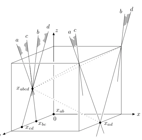
A geometric representation by a linear program
c b
x
y
z
a
a c
b d
d
xabcd
0
xad
xab
xcd
xbc
Figure 5: A linear program inR3essentially representing the square example.
We begin by setting up the following linear program with variables x,y,z (η >0 is a very small positive real number):
minimize z+ηy+η2x subject to a : x+4y−2z ≤ 1
b : 3x+8y+2z ≤ 5
c : 3x−8y+2z ≤ −3
d : −x−4y−2z ≤ −3
x,y,z ≥ 0 .
The corresponding LP-type problem(Hsq,wˆsq)has the set Hsq={a,b,c,d} of four constraints corre-sponding to the four inequalities of the linear program. The value ˆwsq(G)of any subset G⊆Hsqis the minimum of the linear program where the constraints of Hsq\G have been deleted (we stress that the implicit nonnegativity constraints x,y,z≥0 are always present, even for G= /0). In this way, ˆwsq(G)is well defined for every G.
The linear program is illustrated inFigure 5. For better visualization, the picture shows the unit cube[0,1]3, and intersections of the bounding planes of the constraints with the facets x=0 and x=1 of the cube. The minimum of the linear programs containing both the constraints a and c or both the constraints b and d is attained at the point xabcd= (0,1/2,1/2); thus, ˆwsq(Hsq) =1/2. It can be checked that for every subset G of constraints containing neither{a,c}nor{b,d}, the minimum is attained at a point with z=0, and thus with ˆwsq<1/2 (the picture shows the minima for all G of cardinality 2). Thus
ˆ
Next, we observe that if(H,w)is an LP-type problem corresponding to a linear program with vari-ables x1, . . . ,xn and with objective min∑cixi, and(H0,w0) is an LP-type problem corresponding to a linear program with variables x01, . . . ,x0nand with objective min∑c0ix0i, then the join(H,w)∗(H0,w0) cor-responds to the linear program obtained by putting the constraints of both linear programs together and with objective min(∑cixi+∑c0ix0i). Indeed, it suffices to check that the value function in(H,w)∗(H0,w0) coincides with the value function obtained from the combined linear program, and this is immediate. In particular, the m-fold join ˆLm of m disjoint copies of (Hsq,wˆsq) corresponds to the following linear program in 3m variables:
minimize ∑mi=1(zi+ηyi+η2xi)subject to xi+4yi−2zi ≤ 1
3xi+8yi+2zi ≤ 5 3xi−8yi+2zi ≤ −3 −xi−4yi−2zi ≤ −3
xi,yi,zi ≥ 0
i=1,2, . . . ,m .
We could have presented the example forTheorem 1.5in this form, but we find the abstract construction of join more transparent.
Acknowledgment
We would like to thank the anonymous referees for careful reading and a number of valuable comments.
References
[1] *N. AMENTA: Helly theorems and generalized linear programming. Discrete and Computational
Geometry, 12:241–261, 1994. [Springer:bx1262r145x60505]. 1
[2] *N. AMENTA: A short proof of an interesting Helly-type theorem. Discrete and Computational
Geometry, 15:423–427, 1996. [Springer:1fdgptcx3qfd4vm4]. 1
[3] * H. BJORKLUND¨ , S. SANDBERG, AND S. VOROBYOV: A discrete subexponential
algo-rithm for parity games. In Proc. 20th Ann. Symp. on Theoretical Aspects of Computer
Science (STACS’03), Lect. Notes Comput. Sci. 2607, pp. 663–674. Springer-Verlag, 2003.
[Springer:wpjqa08u8db47c3g]. 1
[4] * C. BURNIKEL, K. MEHLHORN, AND S. SCHIRRA: On degeneracy in geometric
computa-tions. In Proc. 5th ACM-SIAM Symp. on Discrete Algorithms (SODA’94), pp. 16–23. SIAM, 1994. [SODA:314464.314474]. 1
[5] * T. CHAN: An optimal randomized algorithm for maximum Tukey depth. In Proc.
15th ACM-SIAM Symp. on Discrete Algorithms (SODA’04), pp. 430–436. SIAM, 2004.
[6] * B. CHAZELLE AND J. MATOUSEKˇ : On linear-time deterministic algorithms for opti-mization problems in fixed dimension. Journal of Algorithms, 21:579–597, 1996. [ Else-vier:10.1006/jagm.1996.0060]. 1
[7] * K. L. CLARKSON: Las Vegas algorithms for linear and integer programming. Journal of the
ACM, 42:488–499, 1995. [JACM:201019.201036]. 1
[8] * H. EDELSBRUNNER AND E. P. M ¨UCKE: Simulation of simplicity: A technique to cope with
degenerate cases in geometric algorithms. ACM Transactions on Graphics, 9(1):66–104, 1990. [ACM:77635.77639]. 1
[9] *I. EMIRIS ANDJ. CANNY: A general approach to removing degeneracies. SIAM J. Computing,
24:650–664, 1995. [SICOMP:10.1137/S0097539792235918]. 1
[10] * K. FISCHER: Smallest enclosing balls of balls. PhD thesis, ETH Z¨urich, Nr. 16168, 2005.
Available athttp://e-collection.ethbib.ethz.ch. 1
[11] * B. G ¨ARTNER, J. MATOUSEKˇ , L. R ¨UST, AND P. ˇSKOVRONˇ: Violator spaces: Structure and
algorithms. Discr. Appl. Math., 2007. In press. Also in arXiv cs.DM/0606087. Extended abstract in Proc. 14th Europ. Symp. Algorithms (ESA’06). [arXiv:cs.DM/0606087]. 1,3
[12] * B. G ¨ARTNER AND I. SCHURR: Linear programming and unique sink orientations. In
Proc. 17th Ann. Symp. on Discrete Algorithms (SODA’06), pp. 749–757. ACM Press, 2006.
[SODA:1109557.1109639]. 1
[13] *B. G ¨ARTNER AND E. WELZL: Linear programming - randomization and abstract frameworks.
In Proc. 13th Ann. Symp. on Theoretical Aspects of Computer Science (STACS’96), pp. 669–687, London, UK, 1996. Springer-Verlag. 1
[14] * B. G ¨ARTNER AND E. WELZL: A simple sampling lemma: Analysis and applications
in geometric optimization. Discrete and Computational Geometry, 25(4):569–590, 2001.
[Springer:9flx12lr0mghtcc4]. 1
[15] *N. HALMAN: On the power of discrete and of lexicographic Helly-type theorems. In Proc. 46th
FOCS, pp. 463–472. IEEE Comp. Soc. Press, 2004. [FOCS:10.1109/FOCS.2004.47]. 1
[16] *J. MATOUˇSEK: On geometric optimization with few violated constraints. Discrete and
Compu-tational Geometry, 14:365–384, 1995. [Springer:r750741557886767]. 1,1,1,2
[17] *J. MATOUSEKˇ , M. SHARIR,ANDE. WELZL: A subexponential bound for linear programming.
Algorithmica, 16:498–516, 1996. [Algorithmica:r378224736133416]. 1
[18] *I. SCHURR: Unique sink orientations of cubes. PhD thesis, ETH Z¨urich, Nr. 15747, 2004. Nr.
15747. Available athttp://e-collection.ethbib.ethz.ch. 1
[19] *M. SHARIR ANDE. WELZL: A combinatorial bound for linear programming and related
prob-lems. In Proc. 9th Symp. on Theoretical Aspects of Computer Science (STACS’92), volume 577 of
[20] *P. ˇSKOVRONˇ: Removing degeneracies in LP-type problems may need to increase dimension. In JANA ˇSAFRANKOV´ A AND´ JIRˇ´IPAVLU˚, editors, Proc. 15th Week of Doctoral Students (WDS), pp.
I:196–207. Matfyzpress, Prague, 2006. 1,3,3
[21] *T. SZABO AND´ E. WELZL: Unique sink orientations of cubes. In Proc. 42nd FOCS, pp. 547–
555. IEEE Comp. Soc. Press, 2001. [FOCS:10.1109/SFCS.2001.959931]. 1
[22] * C. K. YAP: A geometric consistency theorem for a symbolic perturbation scheme. Journal of
Computer and System Sciences, 40(1):2–18, 1990. [JCSS:10.1016/0022-0000(90)90016-E]. 1
AUTHORS
Jiˇr´ı Matouˇsek[About the author]
Department of Applied Mathematics and Institute of Theoretical Computer Science (ITI) Charles University, Malostransk´e n´am. 25 118 00 Praha 1, Czech Republic
matousek kam mff cuni cz
http://kam.mff.cuni.cz/~matousek/
Petr ˇSkovroˇn[About the author] Department of Applied Mathematics Charles University, Malostransk´e n´am. 25 118 00 Praha 1, Czech Republic
xofon kam mff cuni cz
http://kam.mff.cuni.cz/~xofon/
ABOUT THE AUTHORS
JIRˇ´IMATOUSEKˇ has been at Charles University in Prague steadily from 1981 on, although his role there has somehow progressed from student to professor. He has also often enjoyed the hospitality of nice people at many places, most extensively in Berlin, Ger-many and Z¨urich, Switzerland. He has written papers and textbooks in various areas of discrete mathematics and theoretical computer science, such as discrete and compu-tational geometry, low-distortion embeddings of metric spaces, geometric discrepancy, and topological combinatorics, often just out of curiosity. From his youth he has re-tained an aversion towards questionnaires and biographical sketches, although many other things he has already forgotten.