Large‑scale distributed L‑BFGS
Maryam M. Najafabadi
1*, Taghi M. Khoshgoftaar
1, Flavio Villanustre
2and John Holt
2Introduction
A wide range of machine learning algorithms use optimization methods to train the model parameters [1]. In these algorithms, the training phase is formulated as an opti-mization problem. An objective function, created based on the parameters, needs to be optimized to train the model. An optimization method finds parameter values which minimize the objective function. New advances in the machine learning area, such as deep learning [2], have made the interplay between the optimization methods and machine learning one of the most important aspects of advanced computational science. Optimization methods are proving to be vital in order to train models which are able to extract information and patterns from huge volumes of data.
With the recent interest in Big Data analytics, it is critical to be able to scale machine learning techniques to train large-scale models [3]. In addition, recent breakthroughs in representation learning and deep learning show that large models dramatically improve performance [4]. As the number of model parameters increase, classic implementa-tions of optimization methods on one single machine are no longer feasible. Many
Abstract
With the increasing demand for examining and extracting patterns from massive amounts of data, it is critical to be able to train large models to fulfill the needs that recent advances in the machine learning area create. L-BFGS (Limited-memory Broyden Fletcher Goldfarb Shanno) is a numeric optimization method that has been effec-tively used for parameter estimation to train various machine learning models. As the number of parameters increase, implementing this algorithm on one single machine can be insufficient, due to the limited number of computational resources available. In this paper, we present a parallelized implementation of the L-BFGS algorithm on a distributed system which includes a cluster of commodity computing machines. We use open source HPCC Systems (High-Performance Computing Cluster) platform as the underlying distributed system to implement the L-BFGS algorithm. We initially provide an overview of the HPCC Systems framework and how it allows for the parallel and dis-tributed computations important for Big Data analytics and, subsequently, we explain our implementation of the L-BFGS algorithm on this platform. Our experimental results show that our large-scale implementation of the L-BFGS algorithm can easily scale from training models with millions of parameters to models with billions of parameters by simply increasing the number of commodity computational nodes.
Keywords: Large-scale L-BFGS implementation, Parallel and distributed processing, HPCC systems
Open Access
© The Author(s) 2017. This article is distributed under the terms of the Creative Commons Attribution 4.0 International License (http://creativecommons.org/licenses/by/4.0/), which permits unrestricted use, distribution, and reproduction in any medium, provided you give appropriate credit to the original author(s) and the source, provide a link to the Creative Commons license, and indicate if changes were made.
METHODOLOGY
*Correspondence: [email protected]
1 Florida Atlantic University,
777 Glades Road, Boca Raton, FL, USA
applications require solving optimization problems with a large number of parameters. Problems of this scale are very common in the Big Data era [5–7]. Therefore, it is impor-tant to study the problem of large-scale optimizations on distributed systems.
One of the optimization methods, which is extensively employed in machine learning, is Stochastic gradient descent (SGD) [8, 9]. SGD is simple to implement and it works fast when the number of training instances is high, as SGD does not use the whole train-ing data in each iteration. However, SGD has its drawbacks, hyper parameters such as learning rate or the convergence criteria need to be tuned manually. If one is not familiar with the application at hand, it can be very difficult to determine a good learning rate or convergence criteria. A standard approach is to train the model with different param-eters and test them on a validation dataset. The hyperparamparam-eters which give best perfor-mance results on the validation dataset are picked. Considering that the search space for SGD hyperparameters can be large, this approach can be computationally expensive and time consuming, especially on large-scale optimizations.
Batch methods such as L-BFGS algorithm, along with the presence of a line search method [10] to automatically find the learning rate, are usually more stable and easier to check for convergence than SGD [11]. L-BFGS uses the approximated second order gradient information which provides a faster convergence toward the minimum. It is a popular algorithm for parameter estimation in machine learning and some works have shown its effectiveness over other optimization algorithms [11–13].
In a large-scale model, the parameters, their gradients, and the L-BFGS historical vec-tors are too large to fit in the memory of one single computational machine. This also makes the computations too complex to be handled by the processor. Due to this, there is a need for distributed computational platforms which allow parallelized implementa-tions of advanced machine learning algorithms. Consequently, it is important to scale and parallelize L-BFGS effectively in a distributed system to train a large-scale model.
In this paper, we explain a parallelized implementation of the L-BFGS algorithm on HPCC Systems platform. HPCC Systems is an open source, massive parallel-processing computing platform for Big Data processing and analytics [14]. HPCC Systems platform provides a distributed file storage system based on hardware clusters of commodity servers, system software, parallel application processing, and parallel programing devel-opment tools in an integrated system.
Another notable existing large-scale tool for distributed implementations is MapRe-duce [15] and its open source implementation, Hadoop [16]. However, MapReMapRe-duce was designed for parallel processing and it is ill-suited for the iterative computations inher-ent in optimization algorithms [4, 17]. HPCC Systems allows for parallelized iterative computations without the need to add any new framework over the current platform and without the limitation of adapting the algorithm to a specific platform (such as MapReduce key-value pairs).
the whole parameter vector in order to calculate the local gradients on a specific sub-set of data examples. Thus, handling a larger number of parameters requires increasing the memory on each computational node which makes these approaches harder or even infeasible to scale, where the number of parameters are very large. On the other hand, our approach can scale to handle a very large number of parameters by simply increasing the number of commodity computational nodes (for example by increasing the number of instances on an Amazon Web Services cluster).
The remainder of this paper is organized as follows. In section “Related work”, we discuss related work on the topic of distributed implementation of optimization algo-rithms. Section “HPCC systems platform” explains the HPCC Systems platform and how it provides capabilities for a distributed implementation of the L-BFGS algorithm. Sec-tion “L-BFGS algorithm” provides theoretical details of the L-BFGS algorithm. In secSec-tion “Implementation of L-BFGS on HPCC Systems”, we explain our implementation details. In section “Results”, we provide our experimental results. Finally, in section “Conclusion and discussion”, we conclude our work and provide suggestions for future research.
Related work
Optimization algorithms are the heart of many modern machine learning algorithms [19]. Some works have explored the scaling of optimization algorithms to build large-scale models with numerous parameters through distributed computing and paralleliza-tion [9, 18, 20, 21]. These methods focus on linear, convex models where global gradients are obtained by adding up the local gradients which are calculated on each computa-tional node. The main limitation of these solutions is that each computacomputa-tional node needs to store the whole parameter vector to be able to calculate the local gradients. This can be infeasible when the number of parameters is very large. In another study, Niu et al. [22] only focus on optimization problems where the gradient is sparse, meaning that most gradient updates only modify small parts of the parameter vector. Such solu-tions are not general and can only work for a subset of problems.
The research most related to ours are [18] and [4]. Agarwal et al. [18] present a system for learning linear predictors with convex losses on a cluster of 1000 machines. The key component in their system is a communication infrastructure called AllReduce which accumulates and broadcasts values over all nodes. They developed an implementation that is compatible with Hadoop. Each node maintains a local copy of the parameter vec-tor. The L-BFGS algorithm runs locally on each node to accumulate the gradient values locally and the global gradient is obtained by AllReduce. This restricts the parameter vector size to the available memory on only one node. Due to this constraint, their solu-tion only works up to 16 million parameters.
machine, the parameter vector is distributed on many machines which increases the number of parameters that can be stored.
The approach presented in [4] requires a new framework with a parameter server and a coordinator to implement batch optimization algorithms. The approach presented in [18] requires the AllReduce platform on top of MapReduce. However, we do not design or add any new framework on top of the HPCC Systems platform for our implemen-tations. The HPCC Systems platform provides a framework for a general solution for large-scale processing which is not limited to a specific implementation. It allows manipulation of the data locally on each node (similar to the parameter server in [4]). The computational commands are sent to all the computational nodes by a master node (similar to the coordinator approach in [4]). It also allows for aggregating and broadcast-ing the result globally (similar to AllReduce in [18]). Havbroadcast-ing all these capabilities, makes the HPCC Systems platform a perfect solution for parallel and large-scale computations. Since it is an open source platform, it allows practitioners to implement parallelized and distributed computations on large amounts of data without the need to design their own specific distributed platform.
HPCC Systems platform HPCC Systems platform
Parallel relational database technology has proven ineffective in analyzing massive amounts of data [23–25]. As a result, several organizations developed new technologies which utilize large clusters of commodity servers to provide the underlying platform to process and analyze massive data. Some of these technologies include MapReduce [23– 25], Hadoop [16] and the open source HPCC Systems.
MapReduce is a basic system architecture designed by Google for processing and ana-lyzing large datasets on commodity computing clusters. The MapReduce programming model allows distributed and parallelized transformations and aggregations over a clus-ter of machines. The Map function converts the input data to groups according to a key-value pair, and the Reduce function performs aggregation by key-key-value on the output of the Map function. For more complex computations, multiple MapReduce calls must be linked in a sequence.
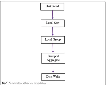
In contrast to MapReduce, in a DataFlow architecture a graph represents a program-ming unit that performs some kind of transformation on the data. Each node in the graph is an operation. Nodes in a graph are connected by edges representing DataFlow queues. Transferring of the data is done by connecting the DataFlow queues. An exam-ple for a DataFlow graph is shown in Fig. 1. First, the data is read from the disk. The next two operations sort and group the data records. Finally some aggregation metrics are extracted from groups of data and the results are written on the disk. This shows how the data is flowing from top to bottom via the connectors of the nodes.
into this model and users need to provide custom MapReduce functions for such opera-tions, which is more error prone and limits re-usability [24].
Some high-level languages, such as Sawzall [26] and Yahoo Pig’s system [27], address some of the limitations of the MapReduce model by providing an external DataFlow-oriented programming language that is eventually translated into MapReduce process-ing sequences. Even though these languages provide standard data processprocess-ing operators so users do not have to implement custom Map and Reduce functions, they are exter-nally implemented and not integral to the MapReduce architecture. Thus, they rely on the same infrastructure and limited execution model provided by MapReduce.
HPCC Systems platform, on the other hand, is an open-source integrated system envi-ronment which excels at both extract, transform and load (ETL) tasks and complex ana-lytics using a common data centric parallel processing language called Enterprise Control Language (ECL). HPCC Systems platform is based on a DataFlow programming model. LexisNexis Risk Solutions1 independently developed and implemented this plat-form as a solution to large-scale data intensive computing. Similar to Hadoop, the HPCC Systems platform also uses commodity clusters of hardware running on top of the Linux operating system. It also includes additional system software and middleware compo-nents to meet the requirements for data-intensive computing such as comprehensive job execution, distributed query and file system support.
1 http://www.lexisnexis.com/.
The data refinery cluster in HPCC Systems (Thor system cluster) is designed for cessing massive volumes of raw data which ranges from data cleansing and ETL pro-cessing to developing machine learning algorithms and building large-scale models. It functions as a distributed file system with parallel processing power spread across the nodes (machines). A Thor cluster can scale from a single node to thousands of nodes. HPCC also provides another type of cluster, called ROXIE [14], for rapid data delivery which is not in the scope of this paper.
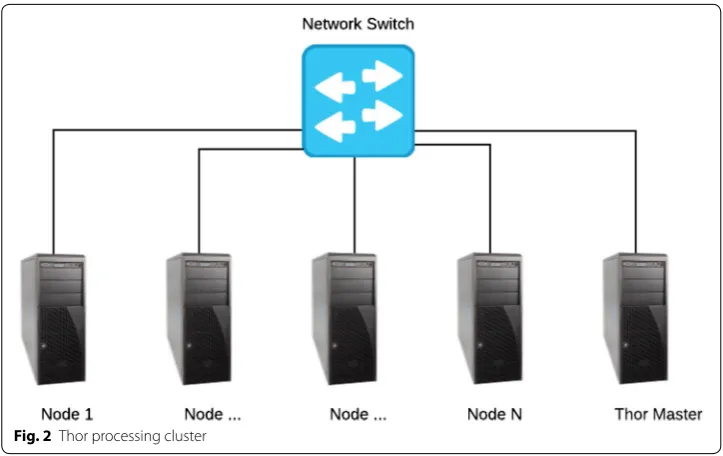
The Thor cluster is implemented using a master/slave topology with a single mas-ter and multiple slave processes, which provide a parallel job execution environment for programs coded in ECL. Each slave provides localized data storage and processing power within the distributed file system cluster. The Thor master monitors and coordi-nates the processing activities of the slave nodes and communicate status information. ECL programs are compiled into optimized C++ source code, which is subsequently linked into executable machine code distributed to the slave processes of a Thor cluster. The distribution of the code is done by the Thor master process. Figure 2 shows a repre-sentation of a physical Thor processing cluster.
The distributed file system (DFS) used in the Thor cluster is record oriented which is somewhat different from the block format used in MapReduce clusters. Each record rep-resents one data instance. Records can be fixed or variable length, and support a variety of standard (fixed record size, CSV, XML) and custom formats including nested child datasets. The files are usually transferred to a landing zone and from there they are parti-tioned and distributed as evenly as possible, with records in sequential order, across the available processes in the cluster.
ECL programming language
The ECL language is a data-centric, declarative language which allows to define paral-lel data processing on HPCC Systems. ECL is a flexible language, where its ease of use
and development speed make HPCC Systems distinguishable from other data-intensive solutions. There are some key benefits with ECL that can be summarized as follows [14]:
• Enterprise Control Language incorporates transparent and implicit data parallelism regardless of the size of the computing clusters reducing the complexity of the paral-lel programming.
• Enterprise Control Language was specifically designed for manipulation of large amounts of data. It enables implementation of data intensive applications with com-plex data-flows and huge volumes of data.
• Since ECL is a higher-level abstraction over C++, it provides more productivity improvements for programmers over languages such as Java and C++. The ECL compiler generates highly optimized C++ for execution.
The ECL programming language is a key factor in the flexibility and capabilities of the HPCC Systems processing environment. ECL is designed following the DataFlow model with the purpose of being transparent and an implicit parallel programming language for data-intensive applications. It is a declarative language which allows the programmer to define the data flow between operations and the DataFlow transformations that are necessary to achieve the results. In a declarative language, the execution is not deter-mined by the order of the language statements, but from the sequence of the operations and transformations in a DataFlow represented by the data dependencies. This is very similar to the declarative style recently introduced by Google TensorFlow [28].
DataFlows defined in ECL are parallelized across the slave nodes which process par-titions of the data. ECL includes extensive capabilities for data definition, filtering and data transformations. ECL is compiled into optimized C++ format and it allows in-line C++ functions to be incorporated into ECL statements. This allows the general data transformation and flow to be represented with ECL code, while the more complex internal manipulations on data records can be implemented as in-line C++ functions. This makes the ECL language distinguishable from other programing languages for data-centric implementations.
Enterprise Control Language transform functions operate on a single record or pair of records at a time depending on the operations. Built-in transform operations in the ECL language which process through entire datasets include PROJECT, ITERATE, ROLLUP, JOIN, COMBINE, FETCH, NORMALIZE, DENORMALIZE, and PROCESS. For exam-ple, the transformation function for the JOIN operation, receives two records at a time and performs the join operation on them. The join operation can be as simple as finding the minimum of two values or as complex as a complicated user-defined in-line C++ function.
L‑BFGS algorithm
Most of the optimization methods start with an initial guess for x in order to minimize an objective function f(x). They iteratively generate a sequence of improving approxi-mate solutions for x until a termination criteria is satisfied. In each iteration, the algo-rithm finds a direction pk and moves along this direction from the current iterate xk to a new iterate xk+1 that has a lower function value. The distance αk to move along pk can be a constant value provided as a hyper-parameter to the optimization algorithm (e.g. SGD algorithm) or it can be calculated using a line search method (e.g. L-BFGS algorithm). The iteration is given by:
where xk is the current point and xk+1 is the new/updated point. Based on the termi-nology provided in [10], pk is called the step direction and αk is called the step length. Different optimization methods calculate these two values differently. Newton optimi-zation methods use the second order gradient information to calculate the step direc-tion. This includes calculating the inverse of the Hessian matrix. In a high dimensional setting, where the parameter vector x is very large, the calculation of the inverse of a Hessian matrix can get too expensive to compute. Quasi Newton methods overcome the problem of calculating the inverse of Hessian matrix in each iteration, by continuously updating an approximation of the inverse of the Hessian matrix in each iteration.
The most popular Quasi Newton algorithm is the BFGS method, named for its dis-coverers, Broyden, Fletcher, Goldfarb, and Shanno [10]. In this method, αk is chosen to satisfy the Wolfe Condition [29] so there is no need to manually select a constant value for αk. The step direction pk is calculated based on an approximation of the inverse of the Hessian matrix. In each iteration, the approximation of the inverse of the Hessian matrix is updated based on the current sk and yk values. Where sk presents the position
difference and yk represents the gradient difference in the iteration. These vectors are the
same length as vector x.
BFGS needs to keep an approximation of the inverse of the Hessian matrix in each itera-tion (an n×n matrix), where n is the length of the parameter vector x. It becomes infea-sible to store this matrix in the memory for large values of n.
The L-BFGS (Limited-memory BFGS) algorithm modifies BFGS to obtain Hessian approximations that can be stored in just a few vectors of the length n. Instead of storing a fully dense n×n approximation, L-BFGS stores just m vectors (m≪n) of length n that
implicitly represent the approximation. The main idea is that it uses curvature informa-tion from the most recent iterainforma-tions. The curvature informainforma-tion from earlier iterainforma-tions are considered to be less likely to be relevant to the Hessian behavior at the current itera-tion and are discarded in the favor of the memory.
In L-BFGS, the {sk,yk} pairs are stored from the last m iteration which causes the
algorithm to need 2×m×n storage compared to n×n storage in the BFGS algorithm. The 2×m memory vectors, along with the gradient at the current point, are used in the
xk+1=xk+αkpk
sk =xk+1−xk
L-BFGS two-loop recursion algorithm to calculate the step direction. The L-BFGS algo-rithm and its two-loop recursion are shown in Algoalgo-rithms 1 and 2, respectively. The next section covers our implementation of this algorithm on HPCC Systems platform.
Algorithm 1 L-BFGS
1: procedureL-BFGS
2: Choose starting pointx0, and integerm >0 3: k←0
4: whiletruedo
5: Calculate∆f(xk)at the current pointxk
6: Calculatepkusing Algorithm 2
7: Calculateαkwhere it satisfies Wolfe conditions
8: xk+1←xk+αkpk
9: ifk > mthen
10: Discard the vector pair{Sk−m, yk−m}from storage 11: end if
12: Compute and Savesk=xk+1−xkandyk= ∆fk+1−∆fk
13: k←k+ 1 14: end while 15: end procedure
Algorithm 2L-BFGS two-loop recursion
1: p← −∆f(xk)
2: fori=k−1, k−2, ..., k−m do
3: αi←si·p/si·yi 4: p←p−αiyi 5: end for
6: p←(sk−1·yk−1/yk−1·yk−1)p
7: fori=k−m, k−m+ 1, ..., k−1 do
8: β←yi·p/si·yi
9: p←p+ (αi−B)si
10: end for 11: returnp
Implementation of L‑BFGS on HPCC Systems Main idea
We used the ECL language to implement the main DataFlow in the L-BFGS algorithm. We also implemented in-line C++ functions as required to perform some local com-putations. We used the HPCC Systems platform without adding any new framework on top of it or modifying any underlying platform configuration.
parameter vector of size 80 GB is broken down to handling only 0.8 GB of partial vectors locally across 100 computational nodes. Even a machine with enough memory to store such a large parameter vector will need even more memory for the intermediate compu-tations and will take a significant amount of time to run only one iteration. Distributing the storage and computations on several machines benefits both memory requirements and computational durations.
The main idea in the implementation of our paralellized L-BFGS alorithm is to dis-tribute the parameter vector over many machines. Each machine manipulates the por-tion of the locally assigned parameter vector. The L-BFGS caches ({si,yi} pairs) are also stored on the machines locally. For example, if the jth machine stores the jth partition of
the parameter vector, it also ends up storing the jth partition of the si and yi vectors by performing all the computations locally. Each machine performs most of the operations independently. For instance, the summation of two vectors that are both distributed on several machines, includes adding up their corresponding partitions on each machine locally.
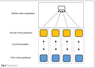
By looking at the L-BFGS algorithm two-loop recursion shown in Algorithm 2, it is clear that all the computations can be performed locally, except the dot product calculation. As mentioned earlier, each machine stores a partition of the parameter vector and all the corresponding partitions of the {si,yi} pairs. Therefore, we calcu-late the partial dot products on each machine locally. We then add up the local dot product results globally to obtain the final dot product result. Figure 3 shows the dot product computation. In the ECL language, a result which is computed by a global aggregation will be automatically accessible on all the nodes locally. There is no need to include any explicit ECL statement in the code to broadcast the global result on all the nodes.
ECL implementation
In this subsection, we explain our implementation using ECL language by providing some examples from the code. The goal is to demonstrate the simplicity of the ECL lan-guage as a lanlan-guage which provides parallelized computations. We refer the interested reader to ECL manual [30] for a detailed explanation of the ECL language.
As mentioned in “HPCC Systems platform”, the distributed file system (DFS) used in a Thor cluster is record oriented. Therefore, we represent each partition of the parameter vector x as a single record. Each record is stored locally on each computational node. Each record consists of several fields. For example, one field represents the node id on which the record is stored. Another field includes the partition values as a set of real numbers. The record definition in ECL language is shown below. It should be noted that since ECL is a declarative language, the := sign implies the declaration and should be read “is defined as”.
x record :=RECORD UNSIGNEDnode id;
SETOF REALpartition values; END;
The record can include other fields as required by the computations. For simplicity, we only show the records related to the actual data and its distribution over several nodes.
The aggregation of the records stored in all the nodes builds a dataset which repre-sents the vector x.
x :=DATASET(...,x record);
The above statement defines vector x as a dataset of records where each record has the x_record format. The “…” includes the actual parameter vector x values which can be a file that contains the initial parameter values or it can be a predefined dataset which is defined in ECL. We exclude that part for simplicity.
Distributing this dataset over several machines is as easy as using a DISTRIBUTE statement in ECL and providing the node_id field as the distribution key. Since we only
have one record per node_id, this means each record is stored on one machine. x distributed :=DISTRIBUTE(x, node id);
x distributed scaled := PROJECT (x distributed, TRANSFORM(...), LO-CAL);
The LOCAL keyword specifies the operation is performed on each computational node independently, without requiring interaction with all other nodes to acquire data. The TRANSFORM(…) defines the type of transformation that should be done on each record. In this case, the SET of real values in the “partition_values” field of each record is multiplied by a constant value and the “node_id” field remains the same. The local com-putations result in the corresponding records from the initial and the result datasets to end up on the same node. All the local computations in our implementation of L-BFGS algorithm are performed in the same manner. This results in the corresponding parti-tions from the L-BFGS cache information vectors, {sk,yk} pairs, the parameter vector itself and its gradient to end up on the same node with the same node_id values, which is important for a JOIN operation as shown below in the dot product operation. The dot product operation can be done using the JOIN statement.
x y dotProduct := JOIN (x distributed, y distributed, LEFT.node id = RIGHT.node id, TRANSFORM(...),LOCAL);
The above statement is joining the two datasets x_distributed and y_distributed where both datasets are distributed over several machines. The JOIN operation is performed locally by pairing the records from the left dataset (x_distributed) and the right data-set (y_distributed) with the same node_id values. The LOCAL keyword results in the two records to be joined locally. The transform function returns the local dot product value for each node_id. Using a simple SUM statement provides the final dot product result. The dot product result can then be used in any operation without any explicit reference to the fact that this is a global value that needs to broadcast to local machines. The HPCC Systems platform implicitly broadcasts such global values on local machines.
Results
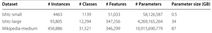
To showcase the effectiveness of our implementation, we consider three different data-sets with increasing number of parameters, lshtc-small, lshtc-large and wikipedia-medium which are large-scale text classification datasets.2 The characteristics of the datasets are shown in Table 1. Each instance in the wikipedia-medium dataset can
2 http://lshtc.iit.demokritos.gr/. Table 1 Dataset characteristics
Dataset # Instances # Classes # Features # Parameters Parameter size (GB)
lshtc-small 4463 1139 51,033 58,126,587 0.5
belong to more than one class. To build the SoftMax objective function, we only consid-ered the very first class among the multiple classes listed for each sample as its label for the wikipedia-medium dataset.
We used the implemented L-BFGS algorithm to optimize the Softmax regression objective function [31] for these datasets. Softmax regression (or multinomial logistic regression) is a generalization of logistic regression for the case where there are multiple classes to be classified. The number of parameters for the SoftMax regression is equal to the multiplication of the number of classes by the number of features. We use dou-ble precision to represent real numbers (8 bytes). The parameter size column in Tadou-ble 1 approximates the memory size which is needed to store the parameter vector by multi-plying the number of parameters by 8. Since the parameter vector is not sparse, we store it as a dense vector which include continuous real values.
We used a cluster of 20 machines, each with 4GB of RAM memory for the lshtc-small dataset. We used an AWS (Amazon Web Service) cluster with 16 instances of r3.8xlarge3 (each instance runs 25 THOR nodes) for lshtc-large and wikipedia-medium datasets where each node has almost 9GB of RAM.
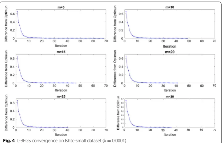
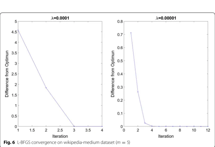
Figure 4 and 5 show the difference from the optimal solution as the number of iter-ations increases for different values of m in the L-BFGS algorithm for lshtc-small and lshtc-large datasets, respectively. We chose the regularization parameter as λ = 0.0001 for these two datasets. We chose a λ value that causes the L-BFGS algorithm not to con-verge as quickly so we can demonstrate more iterations in our results. Figure 6 shows the difference from the optimal solution as the number of iterations increases for m=5 for wikipedia-medium dataset. For this dataset, we chose λ = 0.0001 in addition to λ = 0.0001 because the L-BFGS algorithm converges very fast in the case of λ = 0.0001.
3 https://aws.amazon.com/ec2/instance-types/
The reason we only considered m=5 for this datset is that the number of iteration for the L-BFGS algorithm is small.
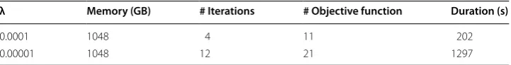
Tables 2, 3, and 4 present the corresponding information for the results shown in Figs. 4, 5, and 6, respectively. The number of iterations is the value where the L-BFGS algorithm reached the optimum point. We define the ending criteria for our L-BFGS algorithm the same as the ending criteria defined in minfunc library [32]. Since in each iteration, the Wolfe line search might need to calculate the objective function more than once to find the best step length, the overall number of times the objective function is
Fig. 5 L-BFGS convergence on lshtc-large dataset (λ = 0.0001)
calculated is usually more than the number of iterations in the L-BFGS algorithm. The total memory usage in these tables presents the required memory by the L-BFGS algo-rithm. It includes the memory required to store the updated parameter vector, the gradi-ent vector, and 2×m L-BFGS cache vectors.
The results indicate that increasing the m value in the L-BFGS algorithm causes the algorithm to reach the optimum point in less number of iterations. However, the time it takes for the algorithm to reach the optimum point does not necessarily decrease. The reason is that increasing m causes the calculation of step direction in L-BFGS two-loop recursion algorithm takes more time.
Our results show that the implemented L-BFGS algorithm on the HPCC Systems can easily scale from handling millions of parameters on dozens of computational nodes to handling billions of parameters on hundreds of machines in a reasonable amount of time. Handling the lshtc-small dataset on 20 computational nodes takes less than 15 min. The lshtc-large dataset with more than 4 billion parameters and the wikipedia-medium dataset with more than 10 billion parameters on a cluster of 400 nodes takes almost 1 h and half an hour, respectively. Although, wikipedia-medium is a larger data-set compared to lshtc-large datadata-set, the L-BFGS algorithm converges in a shorter time, because it requires a smaller number of iterations to reach the optimum.
Table 2 Results description for lshtc‑small dataset
m Memory (GB) # Iterations # Objective function Duration (s)
5 5 68 77 652
10 10 49 58 603
15 15 46 54 668
20 20 41 48 655
25 24 40 46 686
30 29 36 44 641
Table 3 Results description for lshtc‑large dataset
m Memory (GB) # Iterations # Objective function Duration (s)
5 410 61 83 3752
10 751 50 69 3371
15 1093 48 64 3360
20 1434 57 40 2869
25 1776 58 42 3076
30 2117 57 40 3012
Table 4 Results description for wikipedia‑medium dataset
λ Memory (GB) # Iterations # Objective function Duration (s)
0.0001 1048 4 11 202
Conclusion and discussion
In this paper, we explained a parallelized distributed implementation of L-BFGS which works for training large-scale models with billions of parameters. The L-BFGS algorithm is an effective parameter optimization method which can be used for parameter esti-mation for various machine learning problems. We implemented the L-BFGS algorithm on HPCC Systems which is an open source, data-intensive computing system platform originally developed by LexisNexis Risk Solutions. Our main idea to implement the L-BFGS algorithm for large-scale models, where the number of parameters is very large, is to divide the parameter vector into partitions. Each partition is stored and manipu-lated locally on one computational node. In the L-BFGS algorithm, all the computations can be performed locally on each partition except the dot product computation which needs different computational nodes to share their information. The ECL language of the HPCC Systems platform simplifies implementing parallel computations which are done locally on each computational node, as well as performing global computations where computational nodes share information. We explained how we used these capa-bilities to implement L-BFGS algorithm on a HPCC platform. Our experimental results show that our implementation of the L-BFGS algorithm can scale from handling mil-lions of parameters on dozens of machines to bilmil-lions of parameters on hundreds of machines. The implemented L-BFGS algorithm can be used for parameter estimation in machine learning problems with a very large number of parameters. Additionally, It can be used in image or text classification applications, where the large number of features and classes naturally increase the number of model parameters, especially for models such as deep neural networks.
Compared to the parallelized implementation of L-BFGS called Sandblaster, by Google, the HPCC Systems implementation does not require adding any new compo-nent such as a parameter server to the framework. HPCC Systems is an open source platform which already provides the data-centric parallel computing capabilities. It can be used by practitioners to implement their large-scale models without the need to design a new framework. In future work, we want to use the HPCC Systems paralleliza-tion capabilities on each node which is done through multithreaded processing to fur-ther speed up our implementations.
Authors’ contributions
MMN carried out the conception and design of the research, performed the implementations and drafted the manu-script. TMK, FV and JH provided reviews on the manumanu-script. JH set up the experimental framework on AWS and provided expert advice on ECL. All authors read and approved the final manuscript.
Author details
1 Florida Atlantic University, 777 Glades Road, Boca Raton, FL, USA. 2 LexisNexis Business Information Solutions, 245
Peachtree Center Avenue, Atlanta, GA, USA.
Acknowledgements
Not applicable.
Competing interests
The authors declare that they have no competing interests.
Publisher’s Note
Springer Nature remains neutral with regard to jurisdictional claims in published maps and institutional affiliations.
References
1. Bennett KP, Parrado-Hernández E. The interplay of optimization and machine learning research. J Mach Learn Res. 2006;7:1265–81.
2. Najafabadi MM, Villanustre F, Khoshgoftaar TM, Seliya N, Wald R, Muharemagic E. Deep learning applications and challenges in big data analytics. J Big Data. 2015;2(1):1–21.
3. Xing EP, Ho Q, Xie P, Wei D. Strategies and principles of distributed machine learning on big data. Engineering. 2016;2(2):179–95.
4. Dean J, Corrado G, Monga R, Chen K, Devin M, Mao M, Senior A, Tucker P, Yang K, Le QV, et al. Large scale distributed deep networks. In: Advances in neural information processing systems. Lake Tahoe, Nevada: Curran Associates Inc.; 2012. p. 1223–31.
5. Krizhevsky A, Sutskever I, Hinton GE. Imagenet classification with deep convolutional neural networks. In: Pereira F, Burges CJC, Bottou L, Weinberger KQ, editors. Advances in neural information processing systems. Lake Tahoe, Nevada: Curran Associates, Inc.; 2012. p. 1097–05.
6. Dong L, Lin Z, Liang Y, He L, Zhang N, Chen Q, Cao X, Izquierdo E. A hierarchical distributed processing framework for big image data. IEEE Trans Big Data. 2016;2(4):297–309.
7. Sliwinski TS, Kang SL. Applying parallel computing techniques to analyze terabyte atmospheric boundary layer model outputs. Big Data Res. 2017;7:31–41.
8. Shalev-Shwartz S, Singer Y, Srebro N. Pegasos: primal estimated sub-gradient solver for svm. In: Proceedings of the 24th international conference on machine learning. New York: ACM; 2007. p. 807–14.
9. Zinkevich M, Weimer M, Li L, Smola AJ. Parallelized stochastic gradient descent. In: Lafferty JD, Williams CKI, Shawe-Taylor J, Zemel RS, Culotta A, editors. Advances in neural information processing systems. Vancouver, British Colum-bia, Canada: Curran Associates Inc.; 2010. p. 2595–03.
10. Nocedal J, Wright SJ. Numerical optimization. 2nd ed. New York: Springer; 2006.
11. Ngiam J, Coates A, Lahiri A, Prochnow B, Le QV, Ng AY. On optimization methods for deep learning. In: Proceedings of the 28th international conference on machine learning (ICML-11). 2011. p. 265–72.
12. Schraudolph NN, Yu J, Günter S, et al. A stochastic quasi-newton method for online convex optimization. Artif Intell Stat Conf. 2007;7:436–43.
13. Daumé III, H.: Notes on cg and lm-bfgs optimization of logistic regression. http://www.umiacs.umd.edu/~hal/docs/ daume04cg-bfgs, implementation http://www.umiacs.umd.edu/~hal/megam/. 2004; 198: 282.
14. Middleton A, Solutions P. Hpcc systems: introduction to hpcc (high-performance computing cluster). White paper, LexisNexis Risk Solutions. 2011. http://cdn.hpccsystems.com/whitepapers/wp_introduction_HPCC.pdf.
15. Dean J, Ghemawat S. Mapreduce: simplified data processing on large clusters. Commun ACM. 2008;51(1):107–13. 16. White T. Hadoop: the definitive guide. 3rd ed. 2012.
17. Datasets, R.D.: A faulttolerant abstraction for inmemory cluster computing Matei Zaharia, Mosharaf Chowdhury, Tathagata Das, Ankur Dave, Justin Ma, Murphy Mccauley, Michael J. Franklin, Scott Shenker, Ion Stoica University of California: Berkeley.
18. Agarwal A, Chapelle O, Dudík M, Langford J. A reliable effective terascale linear learning system. J Mach Learn Res. 2014;15(1):1111–33.
19. Sra S, Nowozin S, Wright SJ. Optimization for machine learning. Cambridge: The MIT Press; 2011.
20. Dekel O, Gilad-Bachrach R, Shamir O, Xiao L. Optimal distributed online prediction using mini-batches. J Mach Learn Res. 2012;13:165–202.
21. Teo CH, Smola A, Vishwanathan S, Le QV. A scalable modular convex solver for regularized risk minimization. In: Pro-ceedings of the 13th ACM SIGKDD international conference on knowledge discovery and data mining. New York: ACM; 2007. p. 727–36.
22. Recht B, Re C, Wright S, Niu F. Hogwild: a lock-free approach to parallelizing stochastic gradient descent. In: Shawe-Taylor J, Zemel RS, Bartlett PL, Pereira F, Weinberger KQ, editors. Advances in neural information processing systems. Granada, Spain: Curran Associates, Inc.; 2011. p. 693–701.
23. Dean J, Ghemawat S. Mapreduce: a flexible data processing tool. Commun ACM. 2010;53(1):72–7.
24. Chaiken R, Jenkins B, Larson P-Å, Ramsey B, Shakib D, Weaver S, Zhou J. Scope: easy and efficient parallel processing of massive data sets. Proc VLDB Endow. 2008;1(2):1265–76.
25. Stonebraker M, Abadi D, DeWitt DJ, Madden S, Paulson E, Pavlo A, Rasin A. Mapreduce and parallel dbmss: friends or foes? Commun ACM. 2010;53(1):64–71.
26. Pike R, Dorward S, Griesemer R, Quinlan S. Interpreting the data: parallel analysis with sawzall. Sci Program. 2005;13(4):277–98.
27. Gates AF, Natkovich O, Chopra S, Kamath P, Narayanamurthy SM, Olston C, Reed B, Srinivasan S, Srivastava U. Build-ing a high-level dataflow system on top of map-reduce: the pig experience. Proc VLDB Endow. 2009;2(2):1414–25. 28. Abadi M, Agarwal A, Barham P, Brevdo E, Chen Z, Citro C, Corrado GS, Davis A, Dean J, Devin M, et al. Tensorflow:
large-scale machine learning on heterogeneous distributed systems. arXiv preprint. 2016. arXiv:1603.04467. 29. Wolfe P. Convergence conditions for ascent methods. SIAM Rev. 1969;11(2):226–35.
30. Team BRD. Ecl language reference. White paper, LexisNexis Risk Solutions. 2015. http://cdn.hpccsystems.com/install/ docs/3_4_0_1/ECLLanguageReference.pdf.
31. Bishop CM. Pattern recognition and machine learning (information science and statistics). Secaucus: Springer; 2006. 32. Schmidt M. minFunc: unconstrained differentiable multivariate optimization in Matlab. 2005. http://www.cs.ubc.