R E S E A R C H
Open Access
A generalized configuration model with
degree correlations and its percolation
analysis
Duan-Shin Lee
*, Cheng-Shang Chang, Miao Zhu and Hung-Chih Li
*Correspondence: [email protected] Institute of Communications Engineering, National Tsing Hua University, Hsinchu, Taiwan
Abstract
In this paper we present a generalization of the classical configuration model. Like the classical configuration model, the generalized configuration model allows users to specify an arbitrary degree distribution. In our generalized configuration model, we partition the stubs in the configuration model intobblocks of equal sizes and choose a permutation functionhfor these blocks. In each block, we randomly designate a number proportional toqof stubs as type 1 stubs, whereqis a parameter in the range [ 0, 1]. Other stubs are designated as type 2 stubs. To construct a network, randomly select an unconnected stub. Suppose that this stub is in blocki. If it is a type 1 stub, connect this stub to a randomly selected unconnected type 1 stub in blockh(i). If it is a type 2 stub, connect it to a randomly selected unconnected type 2 stub. We repeat this process until all stubs are connected. Under an assumption, we derive a closed form for the joint degree distribution of two random neighboring vertices in the constructed graph. Based on this joint degree distribution, we show that the Pearson degree correlation function is linear inqfor any fixedb. By properly choosingh, we show that our construction algorithm can create assortative networks as well as disassortative networks. We present a percolation analysis of this model. We verify our results by extensive computer simulations.
Keywords: Configuration model, Assortative mixing, Degree correlation
Introduction
Recent advances in the study of networks that arise in field of computer communi-cations, social interactions, biology, economics, information systems,etc., indicate that these seemingly widely different networks possess a few common properties. Perhaps the most extensively studied properties are power-law degree distributions (Barabási and Albert1999), the small-world property (Watts and Strogatz1998), network transitivity or “clustering” (Watts and Strogatz1998). Other important research subjects on networks include network resilience, existence of community structures, synchronization, spread-ing of information or epidemics. A fundamental issue relevant to all the above research issues is the correlation between properties of neighboring vertices. In the ecology and epidemiology literature, this correlation between neighboring vertices is called assortative mixing.
In general, assortative mixing is a concept that attempts to describe the correlation between properties of two connected vertices. Take social networks for example. ver-tices may have ages, weight, or wealthiness as their properties. It is found that friendship between individuals are strongly affected by age, race, income, or languages spoken by the individuals. If vertices with similar properties are more likely to be connected together, we say that the network shows assortative mixing. On the other hand, if vertices with different properties are likely to be connected together, we say that the network shows disassortative mixing. It is found that social networks tend to show assortative mixing, while technology networks, information networks and biological networks tend to show disassortative mixing (Newman2010). The assortativity level of a network is commonly measured by a quantity proposed by Newman (2003) called assortativity coefficient. If the assortativity level to be measured is degree, assortativity coefficient reduces to the standard Pearson correlation coefficient (Newman 2003). Specifically, let X andY be the degrees of a pair of randomly selected neighboring vertices, the Pearson degree correlation function is the correlation coefficient ofXandY, i.e.
ρ(X,Y)def= E(XY)−E(X)E(Y)
σXσY , (1)
whereσX andσY denote the standard deviation ofX andY respectively. We refer the reader to (Newman 2003; 2010; Litvak and van der Hofstad 2012; Xulvi-Brunet and Sokolov2005; Nikoloski et al. 2005; Boguñá et al.2003; Moreno et al.2003) for more information on assortativity coefficient and other related measures. In this paper we shall focus on degree as the vertex property.
complexity ofO(n), wherenis the number of vertices. However, they cannot produce dis-assortatively mixed networks. Users have no explicit control of the level of correlation. Ramezanpour et al. (2005) analyzed the edge-dual graphs of configuration models. They showed that the edge-dual graphs possess non-zero degree correlations and large cluster-ing coefficients. The time complexity of transformcluster-ing a graph to its edge-dual graph is O(m), wheremis the number of edges in the network. However, it seems not possible to tell if the degree correlation is positive or negative analytically. In addition, the degree dis-tribution of the edge-dual graphs can not be determined independently. Newman (2003) and Xulvi-Brunet et al. (2005) proposed algorithms to generate networks with assortative mixing or disassortative mixing by rewiring edges. These algorithms are iteration based and their execution time seems uncontrolled. Bassler et al. (2015) proposed an algorithm to construct a random graph for a given joint degree matrix. The time complexity of the algorithm isO(nm).
In this paper we propose a method to generate random networks that possess either assortative mixing property or disassortative mixing property. Our method is based on a modified construction method of the configuration model. Bender et al. (1978), Bollo´bas (1980) and Molloy et al. (1995;1998) laid down a mathematical foundation for random networks with a given degree distribution. Newman et al. (2001) proposed a construction algorithm for this class of random graphs. Later, graphs so constructed are commonly referred to as the configuration models. Our modified construction method is as follows. Recall that in the construction of configuration models each edge has two “stubs”. We sort and arrange the stubs of all vertices according to degrees. We divide the stubs into blocks and choose a permutation among blocks. To connect stubs, stubs are either randomly connected to a stub in the associated block, or are randomly con-nected to any stub available. The details of our construction algorithm are presented in “Construction of a random network” section. Our method has an advantage that specified degree distributions are preserved in the constructed networks. In addition, our method allows us to derive a closed form for the Pearson degree correlation function for two ran-dom neighboring vertices under an assumption. The time complexity of our construction algorithm isO(m).
The rest of this paper is organized as follows. In “Construction of a random network” section we present our construction method of a random network. In “Joint distribution of degrees” section we derive a closed form for the joint degree distri-bution of two randomly selected neighboring vertices from a network constructed by the algorithm in “Construction of a random network” section. In “Assortativity anddisassor-tativity” section, we show that the Pearson degree correlation function of two neighboring vertices is linear. We then show how permutation functionhshould be selected such that a constructed random graph is associatively or disassortatively mixed. In “An application: percolation” section we present a percolation analysis of this model. Numerical exam-ples and simulation results are presented in “Numerical and simulation results” section. Finally, we give conclusions in “Conclusions” section.
Construction of a random network
Research on random networks was pioneered by Erd˝os and Rényi (1959). Although Erd˝os-Rényi’s model allows researchers to study many network problems, it is limited in that the vertex degree has a Poisson distribution asymptotically as the network grows in size. The configuration model (Bender and Canfield1978; Molloy and Reed1995) can be considered as an extension of the Erd˝os and Rényi model that allows general degree dis-tributions. Configuration models have been used successfully to study the size of giant components. It has been used to study network resilience when vertices or edges are removed. It has also been used to study the epidemic spreading on networks. We refer the readers to (Newman2010) for more details. In this paper we propose an extension of the classical configuration model. This model generates networks with specified degree sequences. In addition, one can specify a positive or a negative degree correlation for the model. Let there benvertices and letpk be the probability that a randomly selected
vertex has degreek. We sample the degree distribution{pk}ntimes to obtain a degree sequencek1,k2,. . .,knfor thenvertices. We give each vertexia total ofkistubs. There
are 2m=ni=1kistubs totally, wheremis the number of edges of the network. In a
clas-sical configuration model, we randomly select an unconnected stub, says, and connect it to another randomly selected unconnected stub in [ 1, 2m]−{s}. We repeat this pro-cess until all stubs are connected. The resulting network can be viewed as a matching of the 2mstubs. Each possible matching occurs with equal probability. The consequence of this construction is that the degree correlation of a randomly selected pair of neighbor-ing vertices is zero. To achieve nonzero degree correlation, we arrange the 2mstubs in ascending order (descending order will also work) according to the degree of the vertices, to which the stubs belong. We label the stubs accordingly. We partition the 2mstubs into bblocks evenly. We select integerbsuch that 2mis divisible byb. Each block has 2m/b stubs. Blocki, wherei=1, 2,. . .,b, contains stubs(i−1)(2m/b)+jforj=1, 2,. . ., 2m/b. Next, we choose a permutation functionhof{1, 2,. . .,b}. Ifh(i)=j, we say that blockjis associated with blocki. In this paper we selecthsuch that
h(h(i))=i,
selected unconnected type 1 stub in blockh(i). If it is a type 2 stub, connect it to a ran-domly selected unconnected type 2 stub in [ 1, 2m]. We repeat this process until all stubs are connected. The construction algorithm is shown in Algorithm 1.
Algorithm 1:Construction Algorithm Inputs: degree sequence{ki:i=1, 2,. . .,n};
Outputs: graph(G,V,E);
Create 2mstubs arranged in descending order;
Divide 2mstubs intobblocks evenly. Initially, all stubs are unconnected. For each block, randomly designate2mq/bstubs as type 1 stubs. All other stubs are designated as type 2 stubs;
whilethere are unconnected stubsdo
Randomly select a stub. Assume that the stub is in blocki; iftype 1 stubthen
connect this stub with a randomly selected unconnected type 1 stub in block h(i);
else
connect this stub with a randomly selected unconnected type 2 stub in [ 1, 2m]; end
end
We make a few remarks.
Remark 1 1. First, note that in networks constructed by this algorithm, there are mq edges that have two type-1 stubs on their two sides. These edges create degree
correlation in the network. On the other hand, there arem(1−q)edges in the
network that have two type-2 stubs on their two sides. These edges do not contribute towards degree correlation in the network. We remark that the graphs produced by our construction algorithm preserve user’s degree distributions.
Under an assumption to be stated in “Joint distribution of degrees” section, we shall
derive a simple expression (Eq. (19)in Theorem2) for the degree correlation
coefficient of the constructed graphs. This expression allows users to specify a targeted level of correlation. Specifically, users choose q to control the magnitude of correlation. Function h controls the sign of correlation coefficients, i.e., assortative mixing versus disassortative mixing.
2. Recall that the ensemble of a random graph consists of all matchings of stubs. For
configuration models, all matchings of stubs are equally likely, which implies that all graphs in the ensemble occur with the same probability. In contrast, the distribution of graphs produced by our construction algorithm is quite
complicated. It requires further investigations in future work. The ensemble of the generalized configuration model consists of groups of random networks. Each group corresponds to a particular assignment of types to stubs. In a particular group in the ensemble, a randomly selected stub connects to another randomly
selected stub in the associated block with probability q. With probability1−q, a
3. Note that standard configuration models can have multiple edges connecting two particular vertices. There can also be edges connecting a vertex to itself. These are called multi-edges and self edges. In our constructed networks, multi-edges and self edges can also exist. However, it is not difficult to show that the expected density of multi-edges and self edges approaches to zero as n becomes large. Due to space limit, we shall not address this issue in this paper.
We also remark that since we allow multi-edges and self edges, our construction algorithm is simple, efficient, and unbiased. If multi-edges and self edges are not allowed, the construction can either take extremely long time or a bias is
introduced. Klein-Hennig et al. (2012) showed that the bias can persist even as
networks grow in size.
Joint distribution of degrees
Consider a randomly selected edge in a random network constructed by the algorithm described in “Construction of a random network” section. In this section we analyze the joint degree distribution of the two vertices at the two ends of the edge.
We randomly select a vertex and letZbe the degree of this vertex. Since the selection of vertices is random,
Pr(Z=ki)= 1 n
fori=1, 2,. . .,n. Thus, the expectation ofZis
E(Z)= n
i=1ki
n =
2m n .
The expectation ofZcan also be expressed as
E(Z)=
∞
k=0
kpk. (2)
The expected number of stubs of the network isE(Z)·n. We would like to evenly allocate these stubs intobblocks such that each block hasnE(Z)/bstubs on average. To provide rigorous mathematical analysis, we make the following assumption.
Assumption 1 The degree distribution{pk}is said to satisfy this assumption if one can find mutually disjoint sets H1,H2,. . .,Hb, such that
b
i=1
Hi= {0, 1, 2,. . .}
and
k∈Hi
kpk =E(Z)/b (3)
for all i=1, 2,. . .,b. In addition, we assume that the degree sequence k1,k2,. . .,kn
sam-pled from the distribution{pk}can be evenly placed in b blocks. Specifically, there exist mutually disjoint sets H1,H2,. . .,Hbthat satisfy
1. bi=1Hi= {1, 2,. . .,n},
2. ki=kjfor anyi∈H1,j∈H2,1=2, and
We randomly select a stub in the range [ 1, 2m]. Denote this stub by t. Let v be the vertex, with which stub t is associated. Let Y be the degree of v. Now con-nect stub t to a randomly selected stub according to the construction algorithm in “Construction of a random network” section. Let this stub be denoted bys. Letube the vertex, with whichsis associated, and letXbe the degree ofu. Since stubtis randomly selected from range [ 1, 2m], the distribution ofYis
Pr(Y =k)= nkpk 2m =
kpk
E(Z), (4)
whereZis the degree of a randomly selected vertex.
To study the joint pmf ofXandY, we first study the conditional pmf ofX, givenY, and the marginal pmfX. In the rest of this section, we assume that Assumption1holds. Supposexis a degree in set Hi. The total number of stubs which are associated with
vertices with degreexisnxpx. By Assumption1, allnxpxstubs are in blocki. We consider
two cases, in which stubtconnects to stubs. In the first case, stubtis of type 1. This occurs with probabilityq. In this case, stubtmust belong to a vertex with a degree in blockh(i). With probability
qnxpx
2mq/b−δi,h(i)
, (5)
the construction algorithm in “Construction of a random network” section connectst to stubs. In (5)δi,j is the Kronecker delta, is equal to one ifi = j, and is equal to zero
otherwise. In the second case, stubtis of type 2. This occurs with probability 1−q. In this case, stubtcan be associated with a degree in any block. With probability
(1−q)nxpx
2m(1−q)−1 (6)
the construction algorithm connects stubtto stubs. Combining the two cases in (5) and (6), we have
Pr(X=x|Y =y)= q
2nxp
x
2mq/b−δi,h(i) +
(1−q)2nxpx
2m(1−q)−1, (7)
fory∈Hh(i). Ify∈Hjforj=h(i),
Pr(X=x|Y =y)= (1−q)
2nxp
x
2m(1−q)−1. (8)
Now assume that the network is large. That is, we consider a sequence of constructed graphs, in whichn→ ∞,m→ ∞, while keeping 2m/n=E(Z). Under this asymptotics, Eqs. (7) and (8) converge to
Pr(X=x|Y =y)→
qb+(1−q)
E(Z) xpx, y∈Hh(i)
1−q
E(Z)xpx, y∈Hj,j=h(i).
(9)
From the law of total probability we have
Pr(X=x) =
y∈Hh(i)
Pr(X=x|Y=y)Pr(Y =y)
+
j=h(i)
y∈Hj
Substituting (4) and (9) into (10), we have
Pr(X=x)=
y∈Hh(i)
qb+(1−q) E(Z) xpx
ypy
E(Z)+
j=h(i)
y∈Hj
1−q E(Z)xpx
ypy
E(Z). (11)
Since the partition of stubs is uniform,
y∈Hj
nypy=2m/b
and thus,
y∈Hj
ypy=E(Z)/b
for anyj=1, 2,. . .,b. Substituting this into (11), we have
Pr(X=x)= xpx
E(Z). (12)
From (9) we derive the joint pmf ofXandY
Pr(X=x,Y =y)=Pr(X=x|Y =y)Pr(Y =y)
=
⎧ ⎪ ⎨ ⎪ ⎩
(bq+1−q) xpx
E(Z) ypy
E(Z),
y∈Hh(i),x∈Hi(1−q)Exp(Zx) ypy
E(Z),
x∈Hi,y∈Hj,j=h(i)
=Cij
xypxpy
(E(Z))2, (13)
where
Cij=
bq+1−q, h(i)=j
1−q, h(i)=j. (14)
We summarize the results in the following theorem.
Theorem 1Let G be a graph generated by the construction algorithm described in “Construction of a random network” section based on a sequence of degrees k1,k2,. . .,kn.
Randomly select an edge fromG. Let X and Y be the degrees of the two vertices at the two ends of the edge. Then, the marginal pmf of X and Y are given in(12)and(4), respectively. The joint pmf of X and Y is given in(13).
Finally, we present some remarks on Assumption1.
Remark 2 1. We first note that Assumption1is very restrictive. It is assumed only for the sake of mathematical cleanness. Distributions functions rarely satisfy this
assumption. Without Assumption1, it is possible that probability masses of some
degrees are across boundaries of blocks. That is, part of some probability masses can be in one block and part of the masses is in a neighboring block. One needs to keep track of how probability masses are split across boundaries. Without
Assumption1, all analyses reported in this paper still can be done. However, the
result can be very messy. This additional complexity not only offers no further insights, but may also clog the readability of this paper. For degree sequences that
do not satisfy Assumption1, the analyses in “Joint distribution of degrees”,
“Assortativity and disassortativity” and “An application: percolation” sections are
simulation results of models constructed without Assumption1with analytical results. We shall see that the difference is very small.
2. We also remark that from (2)one can view
˜
pk=
kpk E(Z)
as a probability mass function. Eq. (3)can be equivalently be expressed as
k∈Hi
˜
pk =1/b
for alli=1, 2,. . .,b. We can equivalently say that distribution{˜pk}satisfies
Assumption1.
3. Finally, we remark that a common way to generate stubs from a degree distribution
is to first generate a sequence of uniform pseudo random variables over[ 0, 1].
Then, transform the uniform random variables using the inverse cumulative
distribution function of the degree distribution (Bratley et al.1987). This approach
would encounter difficulties as far as Assumption1is concerned, because the stubs
produced are not likely to be evenly allocated among blocks. If the network is large, the following approach based on proportionality can be used. Specifically, for
degree k with probability masspk, createnpkvertices andnkpkcorresponding
stubs. If n is large, the strong law of large numbers ensures that this approach and the inversion method produce approximately the same number of stubs. Using this approach, the probability masses of the degree distribution and the stubs sampled
from the degree distribution both satisfy Assumption1and can be placed evenly in
blocks at the same time.
Assortativity and disassortativity
In this section, we present an analysis of the Pearson degree correlation function of two random neighboring vertices. The goal is to search for permutation functionhsuch that the numerator of (1) is non-negative (resp. non-positive) for the network constructed in this section.
From (12), we obtain the expected value ofX
E(X)=
x
xPr(X=x)=
b
i=1
x∈Hi
x2p
x
E(Z) = 1 E(Z)
b
i=1
ui, (15)
where
uidef=
x∈Hi
x2px. (16)
Now we consider the expected value of the productXY. We have from (13) that
E(XY)=
x
y
xyPr(X=x,Y =y)=
b
i=1
b
j=1
x∈Hi
y∈Hj
Cijx2y2pxpy (E(Z))2
=
i
j
Cijuiuj (E(Z))2 =
1
(E(Z))2
⎛
⎝(1−q)
i
j
uiuj+qb
i
uiuh(i)
⎞
Note from (15) and (18) that
E(XY)−E(X)E(Y)= q
(E(Z))2
b
i
uiuh(i)−
i
j
uiuj
. (18)
Based on (18), we summarize the Pearson degree correlation function in the following theorem.
Theorem 2 LetGbe a graph generated by the construction algorithm in “Construction of a random network” section. Randomly select an edge from the graph. Let X and Y be the degrees of the two vertices at the two ends of this edge. Then, the Pearson degree correlation function of X and Y is
ρ(X,Y)=cq, (19)
where
c= b
iuiuh(i)−
i
juiuj σXσY(E(Z))2 ,
andσXandσYare the standard deviation of the pmfs in(12)and(4).
In view of (19), the sign ofρ(X,Y)depends on the constantc. To generate assortative (resp. disassortative) mixing random graphs we sortui’s in descending order first and
then choose the permutationhthat maps the largest number ofui’s to the largest (resp.
smallest) number ofui’s. This is formally stated in the following corollary.
Corollary 1Letπ(·)be the permutation such that uπ(i)is the ithlargest number among ui, i=1, 2,. . .,b, i.e.,
uπ(1)≥uπ(2)≥. . .≥uπ(b).
(i) If we choose the permutation h with h(π(i)) = π(i)for all i, then the constructed random graph is assortative mixing.
(ii) If we choose the permutation h with h(π(i)) = π(b + 1 −i) for all i, then the constructed random graph is disassortative mixing.
The proof of Corollary1is based on the famous Hardy, Littlewood and Pólya rearrange-ment inequality (see e.g., the book Marshall et al. (2011), pp. 141).
Proposition 1(Hardy, Littlewood and Pólya rearrangement inequality)If ui,vi, i=
1, 2,. . .,b are two sets of real number. Let u[i](resp. v[i]) be the ithlargest number among
ui, i=1, 2,. . .,b (resp. vi, i=1, 2,. . .,b). Then
b
i=1
u[i]v[b−i+1]≤
b
i=1
uivi≤ b
i=1
u[i]v[i]. (20)
Proof(Corollary1) (i) Consider the circular shift permutationσj(·)withσj(i)=(i+j− 1 modb)+1 forj=1, 2,. . .,b. From symmetry, we haveσj(i)=σi(j). Thus,
b
i=1
b
j=1
uiuj= b
i=1
b
j=1
uiuσi(j)=
b
j=1
b
i=1
Using the upper bound of the Hardy, Littlewood and Pólya rearrangement inequality in (21) andh(π(i))=π(i)yields
b
i=1
uiuσj(i)≤
b
i=1
u[i]u[i]=
b
i=1
uπ(i)uh(π(i))= b
i=1
uiuh(i). (22)
In view of (18) and (21), we conclude that the generated random graph is assortative mixing.
(ii) Using the lower bound of the Hardy, Littlewood and Pólya rearrangement inequality in (21) andh(π(i))=π(b+1−i)yields
b
i=1
uiuσj(i)≥
b
i=1
u[i]u[b+1−i]=
b
i=1
uπ(i)uh(π(i)) =
b
i=1
uiuh(i). (23)
In view of (18) and (21), we conclude that the generated random graph is disassortative mixing.
An application: percolation
In this section we present a percolation analysis of the generalized configuration model. We consider node percolation of a random network withn vertices. Recall that we defineZto be the degree of a randomly selected vertex in the network. Letpk =Pr(Z=
k)be given and letE(Z)be the expected value ofZ.
Letφ be the probability that a node stays in the network after the percolation. That is, 1 − φ is the probability that a node is removed from the network. In the liter-ature of percolation analysis, φ is called the occupation probability. We assume that
φ ∈ (0, 1). Letαi be the probability that along an edge with one end attached to a stub in blocki, one cannot reach a giant component. Let ηi be the probability that a ran-domly selected vertex from blockiis in a giant component after the random removal of vertices. Then,
ηi=φ k∈Hi
pk
1−αki. (24)
Letηbe the probability that a randomly selected vertex is in a giant component after the random removal of vertices. Then,
η= b
i=1
ηi k∈Hi
pk. (25)
We now derive a set of equations forαi,i=1, 2,. . .,b. We randomly select an edge. Call this edgee. LetDbe the event thatedoes not connect to a giant component. LetBibe the
event that one end of this edge is associated with a stub in blocki. Suppose that the other end ofeis attached to a vertex calledv. Then by the law of total probability we have
Pr(D|Bi)=
b
j=1
∞
k=1
Pr(D|Y =k,Bj,Bi)Pr(Y =k,Bj|Bi), (26)
whereYis the degree ofvandBjis the event that vertexvis in blockj. According to (9),
we have
Pr(Y =k,Bj|Bi)=
qb+(1−q)
E(Z) kpk, k∈Hh(i),
1−q
E(Z)kpk, k∈Hj,j=h(i).
If vertexvis removed from the network through percolation, then edgeedoes not lead to a giant component. This occurs with probability 1−φ. With probabilityφ, vertexvis not removed. Conditioning onY = k, edgeedoes not lead to a giant component if all thek−1 edges ofvdo not. In addition, conditioning onBj, eventDis independent from
eventBi. Combining these facts together, we have
Pr(D|Y=k,Bj,Bi) = Pr(D|Y =k,Bj)
= 1−φ+φαjk−1. (28)
Substituting (27) and (28) into (26), we have
αi = k∈Hh(i)
1−φ+φαkh−(i)1(bq+1−q)kpk E(Z)
+ b
j=1,j=h(i)
k∈Hj
1−φ+φαjk−1(1−q)kpk
E(Z) . (29)
Let
gi(x)=
k∈Hi
kpkxk−1
E(Z) (30)
fori=1, 2,. . .,b. Combining constant terms, we rewrite (29) in terms ofgi(z), i.e.
αi=1−φ+φ ⎛
⎝(bq+1−q)gh(i)(αh(i))+(1−q) b
j=1,j=h(i)
gj(αj) ⎞
⎠. (31)
Expressing (31) in the form of vectors, we have
α=f(α), (32)
whereαis a vector in [ 0, 1]bandf is a vector function that maps from [ 0, 1]bto [ 0, 1]b. In this section, we use boldface letters to denote vectors. Thei-th entry off(α)is denoted by
fi(α)=1−φ+φ ⎛
⎝(bq+1−q)gh(i)(αh(i))+(1−q)
b
j=1,j=h(i)
gj(αj) ⎞
⎠. (33)
Solutions of (32) are called the fixed points of the functionf.
Note thatαi=1 for alli=1, 2,. . .,b, is always a root of (32). Denote point(1, 1,. . ., 1) by1. We are searching for a condition under whichα=1is the only solution of (32) in [ 0, 1]b, and a condition under which (32) has additional solutions. Define
J(a)=
⎛ ⎜ ⎜ ⎜ ⎜ ⎜ ⎝
∂f1(x)
∂x1
∂f1(x)
∂x2 . . .
∂f1(x)
∂xb ∂f2(x)
∂x1
∂f2(x)
∂x2 . . .
∂f2(x)
∂xb
..
. ... . .. ...
∂fb(x) ∂x1
∂fb(x) ∂x2 . . .
∂fb(x) ∂xb
⎞ ⎟ ⎟ ⎟ ⎟ ⎟ ⎠
x=a
, (34)
wherea=(a1,a2,. . .,ab)is a point in [ 0, 1]b. MatrixJ(a)is called the Jacobian matrix of
functionf(x). For functionfdefined in (33), the Jacobian matrix has the following form
J(a)=φ(bqH+(1−q)1b×b)D{g1(a1),g2(a2),. . .,gb(ab)}, (35)
where1b×bis a b×b matrix of unities, andD{g1(a1),g2(a2),. . .,gb(ab)}is a diagonal
|λ1| ≥ |λ2| ≥. . .≥ |λb|.
Sincegjis a power series with non-negative coefficients for allj,gjis strictly increasing
andgj(1) >0. Thus,J(1)is a positive matrix. According to the Perron-Frobenius theorem (Meyer2000; Lancaster and Tismenetsky1985),φλ1is real, positive and strictly larger
thanφλ2in absolute value. In addition, there exists an eigenvectorvassociated with the
dominant eigenvalue that is positive component-wise.
The existence of roots of (32) is summarized in the following main result.
Theorem 3Let
φ=1/λ1. (36)
The solution of (32) can be in one of two cases.
1. If0< φ < φ, point1is an attracting fixed point. In addition, it is the only fixed point in[ 0, 1]b.
2. Ifφ< φ <1, point1is either a repelling fixed point or a saddle point of the
functionf in (32). There exists another fixed point in[ 0, 1)b. This additional fixed
point is an attracting fixed point.
The proof of Theorem3is presented in theAppendix. Note that in case 1 of Theorem3, the only root isα=1. From (24),ηi=0 for alli=1, 2,. . .,b. It follows thatη=0 and the network has no giant component. In case 2, the network has a giant component whose size is determined by the additional fixed point.
We first study the behavior off in the neighborhood of1. We consider the following iteration
xn+1=f(xn), n=0, 1, 2,. . . (37)
where the initial vector x0 is in the neighborhood of the fixed point 1. Assume that
gi(x)can be linearized, i.e.gi(x)can be approximated by keeping two terms in its Taylor expansion around one
gi(x)≈gi(1)+gi(1)(x−1) (38)
for alli=1, 2,. . .,b. Now substituting (38) into (37) and noting that
gi(1)=1/b
(bq+1−q)gh(i)(1)+(1−q)
b
j=1,j=h(i)
gj(1)=1.
for alli=1, 2,. . .,b, we obtain the following matrix equation
xn+1−1=J(1)(xn−1), (39)
where we recall thatJ(1)is the Jacobian matrix stated in (35). Substituting (39) repeatedly into itself, we obtain
xn−1=(J(1))n(x0−1).
If the dominant eigenvalueφλ1<1,xn−1→0and1is an attracting fixed point. If all
are less than one in absolute values. In this case, point1is called a saddle point. Point xnis attracted to1, ifx0−1is a linear combination of the eigenvectors associated with
eigenvalues smaller than one in absolute values. Otherwise,xnmoves away from1.
Numerical and simulation results
We report our simulation results in this section. Recall that we derive the degree covari-ance of two neighboring vertices based on Assumption 1. Assumption 1 is extremely restrictive. For degree sequences that do not satisfy Assumption 1, the analyses in “Joint distribution of degrees” and “Assortativity and disassortativity” sections are only approximate. In this section, we compare simulation results with the analytical results in “Assortativity and disassortativity” section.
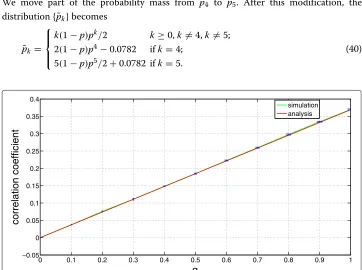
We have simulated the construction of networks with 4000 vertices. We use the batch mean simulation method to control the simulation variance. Specifically, each simulation is repeated 100 times to obtain 100 graphs. Eq. (1) was applied to compute the assorta-tivity coefficient for each graph. One average is computed for every twenty repetitions. Ninety percent confidence intervals are computed based on five averages. We have done extensive number of simulations for uniform and Poisson distributed degree distribu-tions. We have found that simulation results on Pearson degree correlation coefficient agree extremely well with (19) for a wide range ofbandq. Due to space limit, we do not present these results in the paper. We have also simulated power-law degree distributions. Specifically, we assume that the exponent of the power-law distribution is negative two, i.e.,pk ≈k−2for largek. We first fixbat six. The degree correlations for power-law degree
distributions are shown in Figs.1and2for an assortatively mixed network and a disas-sortatively mixed network, respectively. The discrepancy between the simulation result and the analytical result is quite noticeable in Fig.1whenqis large, while the two results agree very well in Fig.2. This is because power-law distributions can generate very large sample values for degrees. As a result, Assumption 1 may fail in this case. We decrease bto two, which increases the block size. The corresponding Pearson degree correlation function for an disassortatively mixed network is presented in Fig.3. One can see that the approximation accuracy is dramatically increased as the block size is increased.
Fig. 2Degree correlation of a disassortative model. Power-law degree distribution andb=6
For percolation analysis, we study the critical value of φ. We assume that degrees are geometrically distributed. However, geometrical distributions do not satisfy Assumption1. Assumption1is essential. Without this assumption,1is not a fixed point and numerical calculations would fail. We must adjust the probability masses to make Assumption1hold. We illustrate this modification for theb=2 case. We start with a geo-metric degree distribution(1−p)pk, wherek=0, 1,. . ., andp=2/3. The corresponding E(Z)=2. We thus have
˜
pk=k(1−p)pk/2, k=0, 1,. . .
We move part of the probability mass from p˜4 to p˜5. After this modification, the
distribution{˜pk}becomes
˜
pk=
⎧ ⎪ ⎨ ⎪ ⎩
k(1−p)pk/2 k≥0,k=4,k=5; 2(1−p)p4−0.0782 ifk=4;
5(1−p)p5/2+0.0782 ifk=5.
(40)
Table 1Critical values ofφ
q=0.2 q=0.5 q=0.8
b=2, assortativity φ 0.22662 0.19518 0.16692
numerical 0.22662 0.19513 0.16688
b=2, disassortativity φ 0.26715 0.29237 0.31231
numerical 0.26711 0.29237 0.31229
b=3, assortativity φ 0.22252 0.18095 0.14540
numerical 0.22251 0.18092 0.14537
b=3, disassortativity φ 0.27442 0.30784 0.32967
numerical 0.27438 0.30782 0.32965
b=3, rotator φ 0.26572 0.29682 0.33182
numerical 0.26571 0.29682 0.33181
Let H1 = {0, 1, 2, 3, 4} and H2 = {k : k ≥ 5}. It is easy to verify that {˜pk} satisfies
Assumption1.
We studyb =2 andb=3. Note that (40) is modified forb =2. Forb= 3, one needs to adjust two probability masses. We omit the details for space reason. In both cases, we study two permutations of blocks suggested in “Assortativity and disassortativity” section for assortativity and disassortativity. For assortative networks,h(i)=i. For disassortative networks,h(i)=b+1−i. In the case ofb=3, we have also studied a rotational permu-tation, i.e.,h(i) = ((i+1) modb)+1. The critical values ofφ obtained using (36) are shown in Table1. We also numerically calculate the critical values ofφ. In this numerical study, we gradually decreaseφuntil (32) fails to have a solution in the interior of [ 0, 1)b. From these results, we see that the critical values ofφobtained from (36) agree very well with those obtained numerically.
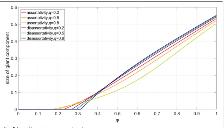
Finally, we study the giant component sizes of the generalized configuration models. We numerically solve (32) to obtain vectorα, and then computeηusing (25). In this study, we continue to assume that degrees are geometrically distributed as we did in the study of Table1. The giant component sizes are shown in Fig.4. From this figure, we see that assortative networks have smaller percolation thresholds than disassortative networks.
Hence, giant components emerge more easily in assortative networks. However, disassor-tative networks tend to have larger giant component sizes than assordisassor-tative networks for largeφ. The effect of assortativity and disassortativity to the giant component sizes and the percolation thresholds observed in this example agrees with that observed in New-man (2002). For the effect ofq, larger values ofq decrease the percolation thresholds and the giant component sizes of assortative networks. On the other hand, larger values ofqincrease the percolation thresholds and the giant component sizes of disassortative networks.
Conclusions
In this paper we have presented an extension of the classical configuration model. Like a classical configuration model, the extended configuration model allows users to specify an arbitrary degree distribution. In addition, the model allows users to specify a positive or a negative assortative coefficient. We derived a closed form for the assortative coefficient of this model. We verified our result with simulations.
Appendix
In this appendix we prove Theorem3. To achieve this, we need a matrix version of the mean value theorem. We state the result in the following lemma.
Lemma 1Suppose thatxandyare two points in[0, 1]b. Then, there exists constants c i
in the open intervals(min(xi,yi), max(xi,yi)), such that
f(x)−f(y)=J(c)(x−y), (41)
wherec=(c1,c2,. . .,cb).
Proof of Lemma1. Suppose thatxandyare two points in [ 0, 1]b. Consider
fi(x)−fi(y) = φ(bq+1−q)gh(i)(xh(i))−gh(i)(yh(i))
+φ(1−q)
b
j=1,j=h(i)
gj(xj)−gj(yj). (42)
Since functiongj is continuous and differentiable in(0, 1), by the mean value theorem
there is acj, where min(xj,yj) <cj<max(xj,yj), such that
gj(cj)= gj(xj)−gj(yj) xj−yj
(43)
for allj. Substituting (43) into (42) and expressing (42) in matrix form, we immediately prove (41).
The proof of Theorem3also needs the Poincaré-Miranda Theorem, which is a ger-eralization of the intermediate value theorem. We quote the Poincaré-Miranda Theorem from (Kulpa1997). LetIb =[ 0, 1]bbe theb-dimensional cube of the Euclidean spaceRb. For eachi≤bdenote
Ii−def= {x∈Ib:xi =0}, Ii+def= {x∈Ib:xi=1}
Proposition 2(Poincaré-Miranda Theorem)Letf :Ib→Rb,f =(f1,f2,. . ., fb), be a
continuous map such that for each i≤ b, fi(Ii−) ⊂ (−∞, 0]and fi(Ii+) ⊂[ 0,+∞). Then, there exists a pointc∈Ibsuch thatf(c)=0.
Now we prove Theorem3.
Proof(Theorem3) Now we analyze the first case in Theorem3. We have shown that fixed point1is attracting. We now show that there is no other fixed point in [ 0, 1]b. Sup-pose not. Assume that there is another distinct fixed point. Denote it byx. From Lemma1, we have
1−x=J(c)(1−x). (44)
Sincegi is a power series with non-negative coefficients,giis monotonically increasing,
differentiable andgiis also increasing. Thus,
J(c) = φ(bqH+(1−q)1b×b)D{g1(c1),g2(c2),. . .,gb(cb)}
≤ φ(bqH+(1−q)1b×b)D{g1(1),g2(1),. . .,gb(1)} (45) = J(1)
component-wise. Inequality (45) is due to the fact thatH,1b×b and the two diagonal
matrices are all non-negative. Substituting the inequality above into (44), we have
1−x≤J(1)(1−x).
Substituting the last inequality repeatedly into itself, we have
1−x≤J(1)n(1−x)→0,
asn→ ∞, since the dominant eigenvalue ofJ(1)is strictly less than one. We thus reach a contradiction to the assumption thatxis distinct from1.
Now we consider the second case. We first show that there exists a pointxin [ 0, 1]b
such that
x−f(x)≥0.
Denote such a point byη. We choose
η=1−v, (46)
where is a small positive number andvis the eigenvalue ofJ(1)associated with the dominant eigenvalueφλ1. For small, we have
f(η)=f(1−v)≈f(1)−J(1)(v)=1−J(1)(v).
It follows from the above equation that
η−f(η)≈(J(1)−I)(v), (47)
whereIis theb×bidentity matrix. Sincevis an eigenvector ofJ(1)associated withφλ1,
(47) reduces to
η−f(η)=(φλ1−1)v.
Sinceφλ1>1 andv>0entry-wise, we have
η−f(η) >0 (48)
Next we shall show that (32) has another fixed point in [ 0, 1)b. To apply Proposition2, we transform system (32) by changing variables. That is, for anyxi∈[ 0,ηi], whereηiis the
i-th entry ofηdefined in (46). We defineyi = xi/ηi, fori = 1, 2,. . .,b. Then, we define
functionF :[ 0, 1]b→[ 0, 1]b, where thei-th entry ofFis
Fi(y)=ηiyi−fi(η1y1,η2y2,. . .,ηbyb).
We now show that for anyy∈Ii−,
Fi(y)
= −fi(η1y1,η2y2,. . .,ηbyb)
= −(1−φ)−φ ⎛
⎝(bq+1−q)gh(i)(ηh(i)yh(i))+(1−q)
j=h(i)
gj(ηjyj) ⎞ ⎠
≤0,
sincegj(ηjyj)≤1/bfor allj. Next, consideryinIi+. In this case,
Fi(y) = ηi−fi(η1y1,. . .,ηi−1yi−1,ηi,ηi+1yi+1,. . .,ηbyb)
≥ ηi−fi(η1,. . .,ηi−1,ηi,ηi+1,. . .,ηb) (49)
≥ 0, (50)
where (49) follows from the monotonicity ofgjfor allj, and (50) follows from (48). From
Proposition2,F(y) = 0has a root in [ 0, 1]b. Equivalently, (32) has a root in [ 0, 1)b. We denote this root byz.
?
We now show that fixed pointzis attracting. From (41) since both1andzare fixed points, we have
1−z=J(c)(1−z), (51)
wherezi<ci<1. From (51), the unity is an eigenvalue ofJ(c)and1−zis the associated
eigenvector. SinceJ(c)is a positive matrix and1−zis a positive vector component-wise, by the Perron-Frobenius theorem, the unity is the dominant eigenvalue ofJ(c) (Meyer 2000). By the definition in (30),giis strictly increasing for alli. It follows thatgi(ci) >gi(zi) and from (35) we have
J(c) = φ(bqH+(1−q)1b×b)D{g1(c1),g2(c2),. . .,gb(cb)}
> φ(bqH+(1−q)1b×b)D{g1(z1),g2(z2),. . .,gb(zb)}
= J(z) (52)
Acknowledgement
This research was supported in part by the Ministry of Science and Technology, Taiwan, R.O.C., under Contract 105-2221-E-007-036-MY3.
Authors’ contributions
DL, CC analyzed the degree correlation and the percolation of the generalized configuration model. MZ performed numerical study on the percolation analysis. HL developed a computer program to simulate the generalized configuration model. All authors read and approved the final manuscript.
Competing interests
The authors declare that we have no competing interests.
Received: 12 August 2019 Accepted: 25 November 2019
References
Barabási A-L, Albert R (1999) Emergence of scaling in random networks. Science 286:509–512
Bassler KE, Genio CID, Erd ˝os PL, Miklós I, Toroczkai Z (2015) Exact sampling of graphs with prescribed degree correlations. New J Phys 17:083052
Bender EA, Canfield ER (1978) The asymptotic number of labelled graphs with given degree sequences. J Comb Theory Ser A 24:296–307
Boguñá M, Pastor-Satorras R (2002) Epidemic spreading in correlated complex networks. Phys Rev E 66:047104 Boguñá M, Pastor-Satorras R, Vespignani A (2003) Absence of epidemic threshold in scale-free networks with degree
correlations. Phys Rev Lett 90:028701
Bollobás B (1980) A probabilistic proof of an asymptotic formula for the number of labelled regular graphs. Eur J Comb 1:311–316
Braha D (2016) The complexity of design networks: Structure and dynamics. In: Cash P, Mario TS, Štorga (eds). Experimental Design Research. pp 129–151.https://doi.org/10.1007/978-3-319-33781-4_8
Braha D, Bar-Yam Y (2007) The statistical mechanics of complex product development: Empirical and analytical results. Manag Sci 53(7):1127–1145
Bratley P, Fox BL, Schrage LE (1987) A Guide to Simulation, 2nd edn. Springer, New York
Callaway DS, Hopcroft JE, Kleinberg JM, Newman MEJ, Strogatz SH (2001) Are randomly grown graphs really random? Phys Rev E 64:041902
Cardy JL, Grassberger P (1985) Epidemic models and percolation. J Phys A Math Gen 18(6):L267–L271.https://doi.org/10. 1088/0305-4470/18/6/001.https://doi.org/10.1088%2F0305-4470%2F18%2F6%2F001
Catanzaro M, Caldarelli G, Pietronenero L (2004) Assortative model for social networks. Phys Rev E 70:037101 Cohen R, Erez K, ben-Avraham D, Havlin S (2000) Resilence of the internet to random breakdowns. Phys Rev Lett
85:4626–4628
Eguíluz VM, Klemm K (2002) Epidemic threshold in structured scale-free networks. Phys Rev Lett 89(10, 108701):108701. https://doi.org/10.1103/PhysRevLett.89.108701
Erd ˝os, Rényi (1959) On random graphs. Publ Math 6:290–297
Guiver C (2018) On the strict monotonicity of spectral radii for classes of bounded positive linear operators. Positivity 22:1173–1190
Johnson S, Torres JJ, Marro J, Munoz MA (2010) The entropic origin of disassortativity in complex networks. Phys Rev Lett 104:108702
Klein-Hennig H, Hartmann AK (2012) Bias in generation of random graphs. Phys Rev E 85:026101 Kulpa W (1997) The Poincaré-Miranda theorem. Am Math Mon 104(6):545–550
Lancaster P, Tismenetsky M (1985) The Theory of Matrices. Academic Press, New York
Litvak DN, van der Hofstad R (2012) Degree-degree correlations in random graphs with heavy-tailed degrees.
Department of Applied Mathematics, University of Twente, Enschede, the Netherlands.http://doc.utwente.nl/84367/ Marshall AW, Olkin I, Arnold BC (2011) Inequalities: Theory of Majorization and Its Applications. Springer, New York Meyer C (2000) Matrix Analysis and Applied Linear Algebra. SIAM, Philadelphia, USA
Molloy M, Reed B (1995) A critical point for random graphs with a given degree sequence. Random Struct Alg 6:161–179 Molloy M, Reed B (1998) The size of the giant component of a random graph with a given degree sequence. Comb
Probab Comput 7:295–306
Moore C, Newman MEJ (2000) Epidemics and percolation in small-world networks. Phys Rev E 61:5678
Moreno Y, Gómez JB, Pacheco AF (2003) Epidemic incidence in correlated complex networks. Phys Rev E 68:035103 Newman MEJ (2001) Clustering and preferential attachment in growing networks. Phys Rev E 64:025102
Newman MEJ (2002) Assortative mixing in networks. Phys Rev Lett 89:208701 Newman MEJ (2003) Mixing patterns on networks. Phys Rev E 67:026126 Newman M (2010) Networks: An Introduction. Oxford University Press, New York
Nikoloski Z, Deo N, Kucera L (2005) Degree-correlation of a scale-free random graph process. In: Stefan F (ed). 2005 European Conference on Combinatorics, Graph Theory and Applications (EuroComb ’05) Vol. AE. pp 239–244.http:// www.dmtcs.org/proceedings/html/dmAE0148.abs.html
Pomerance A, Ott E, Girvan M, Losert W (2009) The effect of network topology on the stability of discrete state models of genetic control. Proc Natl Acad Sci 106:8209–8214
Ramezanpour A, Karimipour V, Mashaghi A (2005) Generating correlated networks from uncorrelated ones. Phys Rev E 67:046107
Sander LM, Warren CP, Sokolov IM, Simon C, Koopman J (2002) Percolation on heterogeneous networks as a model for epidemics. Math Biosci 80:293–305
Schwartz N, Cohen R, ben-Avraham D, Barabasi A-L, Havlin S (2002) Percolation in directed scale-free networks. Phys Rev E 66:015104
Schläpfer M, Buzna L (2012) Decelerated spreading in degree-correlated networks. Phys Rev E 85:015101 Vázquez A, Moreno Y (2003) Resilence to damage of graphs with degree correlations. Phys Rev E 67:015101 Watts DJ, Strogatz SH (1998) Collective dynamics of ’small-world’ networks. Nature 393:440–442
Xulvi-Brunet R, Sokolov IM (2005) Changing correlations in networks: assortativity and dissortativity. Acta Phys Pol B 36(5):1431–1455
Zhou J, Xu X, Zhang J, Sun J, Small M, Lu J-A (2008) Generating an assortative network with a given degree distribution. Intern J Bifuration Chaos 18(11):3495–3502
Publisher’s Note