On the statistical performance of Granger-causal connectivity estimators

(1)

On the statistical performance of Granger-causal connectivity

estimators

Koichi Sameshima•_{Daniel Y. Takahashi} •_{Luiz A. Baccala´}

Received: 23 January 2015 / Accepted: 23 March 2015 / Published online: 22 April 2015 ÓThe Author(s) 2015. This article is published with open access at Springerlink.com

Abstract In this article, we extend the statistical detection performance evaluation of linear connectivity from Sameshima et al. (in: Slezak et al. (eds.) Lecture Notes in Computer Science, 2014) via brand new Monte Carlo simulations of three widely used toy models under different data record lengths for a classic time domain multivariate Granger causality test, information partial directed coher-ence, information directed transfer function, and include conditional multivariate Granger causality whose be-haviour was found to beanomalous.

Keywords Partial directed coherenceDirected transfer function Granger causalityNull hypothesis test performance Conditional multivariate Granger causality

1 Introduction

This paper compares the statistical performance of linear connectivity detection [1] using four popular neural con-nectivity estimators. In addition to the classic Gran-ger causality test (GCT) from [2], we employ our recently derived rigorous results [3, 4] about the asymptotic

behaviour of information PDC (iPDC) and information DTF (iDTF) [5] that, respectively, generalize partial di-rected coherence (PDC) [6] and directed transfer function (DTF) [7] which correctly describe coupling effect size issues. A fourth method was included in this extended version of [8] and consists of the proposal put forward by [9] (cMVGC) for detecting conditional Granger causality between time series pairs and is applied here using their published MVGC package. There have been many recent papers [10–14] aimed at comparing contending connec-tivity estimation procedures. In fact, almost every new connectivity estimation procedure sports some form of appraisal by counting the number of correct detection de-cisions. What sets the present effort apart, as emphasized by using the wordstatistical, is that we focus on methods that have rigourous theoretically derived asymptotic de-tection criteria.

In the comparisons, we used Monte Carlo simulations of three widely used toy models from the literature and ver-ified the performance of null connectivity hypothesis re-jection as a function of data record length, K. To complement the study, we also computed false positive (FP) and false negative (FN) test rates for each estimator alternative. In the MVGC package case, false detection rates were computed with and without author-recom-mended corrections [9].

2 Methods and results

2.1 Monte Carlo simulations

Following our recently proposed information PDC and information DTF [5], and their corresponding rigorous asymptotic statistics (see [3] and [4] for details), we first K. Sameshima (&)

Radiology & Oncology Department, Faculdade de Medicina, University of Sa˜o Paulo, Sa˜o Paulo, SP 01246-903, Brazil e-mail: [email protected]

D. Y. Takahashi

Psychology Department, Neuroscience Institute, Princeton University, Princeton, NJ, USA

L. A. Baccala´

(2)

gauged their statistical performance against that of the well-established time-domain GCT test [2]. For added comparison here, we added results from conditional con-nectivity detection obtained via the MVGC package [9]. Monte Carlo simulations were performed in the MATLAB environment using its normally distributed pseudorandom number generator to simulate systems with uncorrelated zero mean and unit variance innovation noise as model

inputs. To test the performance of the latter four connec-tivity estimators, for each toy model and at each data record length, we selected values of K={100, 200, 500, 1000, 2000, 5000, 10000} repeating 1000 simulations for each case. For each simulation, a burn-in set of 5000 initial data points were discarded to eliminate possible transients before selecting the K value of interest. We used the Nuttall-Strand algorithm for multivariate autoregressive (MAR) model estimation and the Akaike information cri-terion (AIC) for model order selection [15] for GCT,iPDC andiDTF, while the Levinson–Wiggins–Robinson solution of the multivariate Yule-Walker equations was used as is default for cMVGC [9]. Detection threshold was set in compliance toa¼1%. ForiPDC andiDTF, pvalues were computed at 32 uniformly separated normalized frequency points covering the whole interval with a connection being deemed detected for a given pair of structures if its pvalue resulted to be less than a for some frequency within the interval. This connectivity decision criterion is somewhat lax and tends to overestimate the presence of connectivity for iPDC and iDTF. In particular for iPDC, one should

1 3

2

4 5

6 7

Fig. 1 Diagram depicting the essential elements of Model 1

represented by Eq.1from [16]. The elements fromx1tox5establish

closed-loop connections, with short and long connected paths, while

x6 and x7 are part of a completely separate substructure, i.e.

disconnected fromfx1;. . .;x5g, but sharing a common frequency of

oscillation

i

PDC

1 2 3 4 5 6 7

1

2

3

4

5

6

7

1

2

3

4

5

6

7

1 2 3 4 5 6 7

i

DTF

0.5 1 0 0.5 1 0 0.5 1 0 0.5 1 0 0.5 1 0 0.5 1 0 0.5 1

0.5 1 0 0.5 1 0 0.5 1 0 0.5 1 0 0.5 1 0 0.5 1

log Spectra [a.u.]

0 0.5 1

0.5 1 0 0.5 1 0 0.5 1 0 0.5 1 0 0.5 1 0 0.5 1 0 0.5 1

0.5 1 0 0.5 1 0 0.5 1 0 0.5 1 0 0.5 1 0 0.5 1

log Spectra [a.u.]

0 0.5 1

(c)

(b)

(a)

(d)

0 1

0 .5

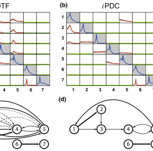
Fig. 2 A single-trial results of a iDTF and b iPDC estimations

obtained using a data simulation of Model 1 with K=2000 points. In both subfigures, a, b, the main diagonal subplots with gray backgroundcontain power spectra, while each off-diagonal subplot represents iDTF or iPDC measure in the frequency domain with variables incolumnsrepresenting the sources and in rows the target structures, in which significant measure is drawn in red lines at

a¼1%, and in green linesotherwise.cNote that, as theoretically expected, according to iDTF estimation, all nodes of fx1;x2;x3;x4;x5gset can reach one another,dwhileiPDC correctly

exposes, similar to GCT, the immediate adjacent node’s connectivity pattern. See further discussion about the contrast betweeniDTF and

(3)

expect connectivity detection more often than GCT, i.e. more FPs are likely.

The reader may access our open MATLAB codes for GCT and for both iPDC and iDTF asymptotic statistics used in this study at http://www.lcs.poli.usp.br/*baccala/ BIHExtension2014/.

The Web site, furthermore, contains the datasets of the employed simulation results and a copy of the exact ver-sion of the MVGC package used in the present compar-isons [9]. This allows full reader accessing disclosure of the data/procedures with the possibility of cross-checking and replaying all results. Additional graphs and results are available there and may be consulted for details; only the overall representative behaviour is summed up here.

Next we describe the toy models and the allied simulations results.

2.2 Model 1: Closed-loop model

It is an fN¼7g-variable model, borrowed from [16] (Fig.1), with two completely disconnected substructures,

{x1;x2;x3;x4;x5} and {x6, x7}, which share a common frequency of oscillation. The set of descriptive equations is

x1ðtÞ ¼ 0:95

ffiffiffi 2

p

x1ðt1Þ 0:9025x1ðt2Þ

þ 0:5x5ðt2Þ þw1ðtÞ

x2ðtÞ ¼ 0:5x1ðt1Þ þw2ðtÞ

x3ðtÞ ¼ 0:2x1ðt1Þ þ0:4x2ðt2Þ þw3ðtÞ

x4ðtÞ ¼ 0:5x3ðt1Þ þ0:25

ffiffiffi 2

p

x4ðt1Þ

þ 0:25pffiffiffi2x5ðt1Þ þw4ðtÞ

x5ðtÞ ¼ 0:25

ffiffiffi 2

p

x4ðt1Þ þ0:25

ffiffiffi 2

p

x5ðt1Þ þw5ðtÞ

x6ðtÞ ¼ 0:95

ffiffiffi 2

p

x6ðt1Þ 0:9025x6ðt2Þ þw6ðtÞ

x7ðtÞ ¼ 0:1x6ðt2Þ þw7ðtÞ;

8 > > > > > > > > > > > > > > > > > > > > > > < > > > > > > > > > > > > > > > > > > > > > > :

ð1Þ

where wi stand for uncorrelated N ð0;1Þ Gaussian

innovations.

10

(

p

)

GCT

1

0 2 4

0 2 4 6

0 5 10 15

0 2 4

0 5 10 15

2

0 2 4 6 8

0 2 4

0 2 4 6

0 2 4

0 5 10 15

3

0 2 4

0 2 4 6

0 2 4

0 2 4 6

0 2 4

0 5 10 15

4

0 5 10 15

0 2 4 6

0 2 4

0 5 10 15

5

0 2 4 6

0 2 4

6

0 2 4

0 5 10

100 200 500100020005000₁₀₀₀₀

0 2 4 6

0 2 4

0 2 4 6

0 5 10 15

7

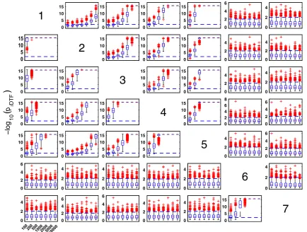
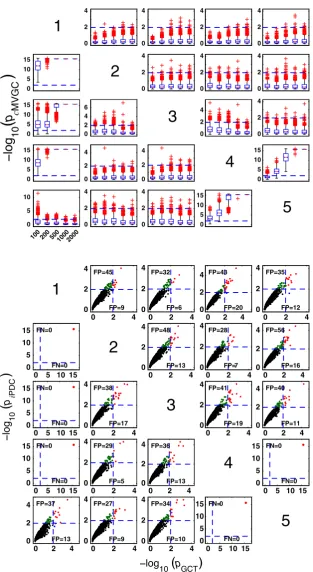
Fig. 3 The patterns (in this and all the figures of similar kind that

follow) containing subplots with variables in columns representing the sources and the target structures in rows. Each subplot possesses boxplots of the distribution of GCT-log10(pvalue) for 1000 Monte

Carlo simulations over different record lengths K={100, 200, 500,

1000, 2000, 5000, 10000} along the x-axis of each subplot. Since

(4)

Results from a single-trial example ofiDTF andiPDC connectivity estimations in the frequency domain are de-picted in Fig.2a, b, respectively, with significant values, at a¼0:01, represented by red solid lines. The corre-sponding connectivity graph diagrams are contained in Fig.2c, d, where arrow thickness represents estimate magnitude. Note thatiPDC reflects adjacent connections, Fig.2b, d, while iDTF, Fig.2a, c, represents graph reachability aspects of the directed structure [17,18]. The notion of reachability refers to the net influence from a time series onto another through various signal pathways, i.e. it measures how much of one series ends up influ-encing another.

2.2.1 Granger causality test for Model 1

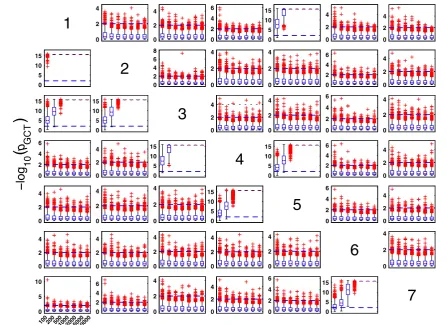
The boxplots of-log10(pvalue) in Fig. 3summarize GCT

performance for Model 1 and K={100, 200, 500, 1000, 2000, 5000, 10000} data record lengths. As expected, for

K[200, it properly detects connectivity between adjacent structures with zero observed FNs for all pairs of existing connections.

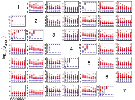
2.2.2 iPDC performance for Model 1

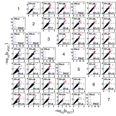
Figure4 summarizes the asymptoticiPDC statistical per-formances for the same data and record lengths as for GCT in Fig. 3 with similar performance (Figs. 5, 6). Closer comparison on identical trials for each estimator leads to Fig.7 depicting iPDC versus GCT performance (K=2000), further revealing a pattern of consistently higher FP values foriPDC expectedly resulting from how the test was performed with iPDC decision dictated by a single maximum frequency above threshold. In Fig.7, the average slopes are above 45° consistent with the larger number of FPs foriPDC.

At this point, one should note that for trial-by-trial comparisons between methods only those against GCT are present for the sake of conciseness. Pairwise behaviour for other pairs of methods is easy to infer. GCT’s choice as a reference was dictated by its canonical behaviour in terms of the expected performance in the Neyman–Pearson hy-pothesis testing framework. In the Web site, it is possible to use available routines to examine the results that apply to the comparison between other pairs of methods.

10

(

p

iPDC

)

7

0 5 10 15

0 2 4

0 2 4 6

0 2 4

0 2 4 6 8

0 5 10

100 200 500100020005000₁₀₀₀₀

0 2 4

6

0 2 4

0 2 4 6

5

0 5 10 15

0 2 4

0 2 4 6

0 5 10 15

4

0 5 10 15

0 2 4

0 2 4 6

0 2 4

0 2 4 6

0 2 4

0 2 4 6

3

0 5 10 15

0 2 4 6

0 2 4 6 8

0 2 4

0 2 4 6

2

0 5 10 15

0 2 4 6

0 5 10 15

0 2 4 6

0 2 4

1

(5)

2.2.3 cMVGC behaviour for Model 1

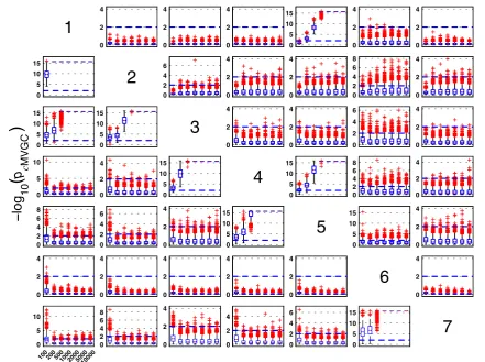
Figure5summarizes the performance of pairwise conditional MVGC in the form of boxplots. They asymptotically capture the structure of Fig.1despite differences compared to GCT andiPDC. These differences are easier to appreciate on the trial-by-trial comparison with respect to GCT (Fig.8), which shows thatcMVGC’s FP rates are sometimes well below the imposeda¼1% and even become more extreme after au-thors’ recommended corrections [9] (K=2000). Note how point distributions in Fig.8hardly ever cluster round the 45°

line for connections reaching thex1 andx6 oscillators. For connections leavingx6, the pattern is reversed. It is this failure to meet the preseta¼1%irrespective of which connection is under consideration, which we callanomaloushere.

2.2.4 iDTF performance for Model 1

Figure6 summarizes the performance of the asymptotic statistics for iDTF. The boxplots clearly show that for larger sample sizes,iDTF correctly detects the reachability structure shown in Fig.2c. Note that the weakest, and in

this case, the farthest connection (x2!x1) requires longer record lengths for proper detection.

2.3 Model 2: Five-variable model

Model 2 introduced by [6] is graphically represented in Fig.9with its corresponding set of defining equations:

x1ðtÞ ¼ 0:95

ffiffiffi 2

p

x1ðt1Þ 0:9025x1ðt2Þ þw1ðtÞ

x2ðtÞ ¼ 0:5x1ðt2Þ þw2ðtÞ x3ðtÞ ¼ 0:4x1ðt3Þ þw3ðtÞ

x4ðtÞ ¼ 0:5x1ðt2Þ þ0:25

ffiffiffi 2

p

x4ðt1Þ

þ 0:25pffiffiffi2x5ðt1Þ þw4ðtÞ

x5ðtÞ ¼ 0:25

ffiffiffi 2

p

x4ðt1Þ þ0:25

ffiffiffi 2

p

x5ðt1Þ þw5ðtÞ;

8 > > > > > > > > > > > > < > > > > > > > > > > > > :

ð2Þ

where wi, as before, stand for uncorrelated Gaussian

in-novations. Computations were performed for K={100, 200, 500, 1000, 2000} long records over 1000 Monte Carlo repetitions.

10

(

p

c

MVGC

)

7

0 5 10 15

0 2 4 6

0 2 4

0 2 4 6 8

0 5 10

100 200 500100020005000₁₀₀₀₀

0 2 4

6

0 2 4

0 5 10 15

5

0 5 10 15

0 2 4

0 2 4 6

0 2 4 6 8

0 2 4

0 2 4 6 8

0 5 10 15

4

0 5 10 15

0 2 4

0 5 10

0 2 4

0 2 4 6

0 2 4

3

0 5 10 15

0 2 4

0 2 4 6 8

0 2 4

0 2 4 6

2

0 5 10 15

0 2 4

0 5 10 15

0 2 4

1

Fig. 5 Model 1 boxplot performance summary ofcMVGC

asymp-totics. Note thatred crossoutliers for the connections intox1andx6

(see the firstand sixth rowsof subplots’ layouts) are consistently

below-log10(pvalue)=2, and those fromx6consistently above for

(6)

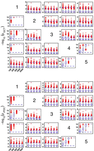
2.3.1 GCT performance

As before, Model 2 also shows that GCT’s performance improves with the increased record length (Fig.10). At

K=200, GCT already performs well with FN rate below 5 %, reaching overall FN rates below 2 % for K=2000.

2.3.2 iPDC performance

For Model 2, FN rates are practically negligible whenK[

200 for all measures of GCT, iPDC, and cMVGC (See Figs.10–12). Overall, the pattern ofiPDC performance is similar to that of GCT’s. YetiPDC’s FP rates are slightly higher than GCT’s. For example, performance for

K=2000 is between 2.7 and 5.6 % (Fig.13).

2.3.3 cMVGC asymptotic behaviour for Model 2

cMVGC performance for K={100, 200, 500, 1000, 2000} is shown in Fig.12. When taken with respect to GCT (Fig. 14), FPs are consistently lower than GCT’s for K=2000 and, as in the case of the previous model, it does

not conform to a preseta¼1% for FP rates. This is also easy to appreciate for other values ofK in Fig.12as most outliers (red crosses) are below the -log10(p value)=2

line for nonexisting connections.

Taking GCT as a reference, trial-by-trial comparisons of

iPDC and cMVGC, respectively, confirm the pattern of higher FP for the former compared to a pattern of FP, below 1 %, for cMVGC with or without correction (See Figs. 13,14). This is also suggestive of possible problems encountered in how the MVGC package handles the FP rate, which may be fortuitously benign to MVGC in this example, but does not represent the general case, since it does not hold for Model 1.

2.4 Model 3: Modified five-var model

To further probe the statistical behaviours of GCT, iPDC and cMVGC, we simulated the modified five-channel toy Model 3, originally introduced in [6], under the formula-tion variant proposed by [19] and reproduced here for reference (Fig.15).

The corresponding set of equations is

10

(

p iDTF

)

7

0 5 10 15

0 2 4

0 2 4 6

0 2 4

100200500100020005000₁₀₀₀₀

0 2 4

6

0 2 4

0 2 4 6

0 2 4

5

0 5 10 15

0 2 4 6

0 2 4 6 8

0 5 10 15

4

0 5 10 15

0 2 4

0 5 10 15

3

0 5 10 15

0 2 4

0 5 10 15

2

0

5 10 15

0 2 4

0 2 4 6

0 5 10 15

1

Fig. 6 Model 1 boxplot performance summary ofiDTF asymptotics. Note that every node offx1;x2;x3;x4;x5gset can directionally reach one

(7)

x1ðtÞ ¼ 0:95

ffiffiffi 2

p

x1ðt1Þ 0:9025x1ðt2Þ

þe1ðtÞ þa1e6ðtÞ þb1e7ðt1Þ þc1e7ðt2Þ

x2ðtÞ ¼ 0:5x1ðt2Þ

x3ðtÞ ¼ 0:4x1ðt3Þ

x4ðtÞ ¼ 0:5x1ðt2Þ þ0:25

ffiffiffi 2

p

x4ðt1Þ þ0:25

ffiffiffi 2

p

x5ðt1Þ

x5ðtÞ ¼ 0:25

ffiffiffi 2

p

x4ðt1Þ þ0:25

ffiffiffi 2

p

x5ðt1Þ

þe5ðtÞ þa5e6ðtÞ þb5e7ðt1Þ þc5e7ðt2Þ;

8 > > > > > > > > > > > > > > > > > > > > > > > > > < > > > > > > > > > > > > > > > > > > > > > > > > > :

ð3Þ

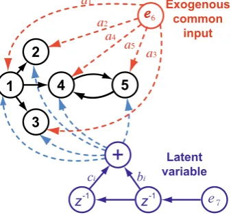
additionally containing the large exogenous inpute6ðtÞand the latent variable e7ðtÞ. In the simulations, eiðtÞ were uncorrelated zero mean unit variance Gaussian innovation

noises, and the parameters were chosen as

aiUð0;1Þ;bi¼2 and ci¼5;i¼1;. . .;5 according to

[19].

The proposal in [19] of introducing exogenous/latent variables is an interesting idea which allows investigating the influence of large common additive noise sources on the performance of GCT, iPDC and cMVGC. Here, to assess the impairment that the extra exogenous/latent variables possibly inflict on null-hypothesis testing, we repeated the procedure not just under the same conditions of [19], but also using a broader range of data record sizes:

K¼ f100;200;500;1000;2000;5000;10000g:

2.4.1 GCT performance in the presence of exogenous noise, Model 3

The GCT performance for Model 3 can be appreciated in Fig.16. When compared with Model 2, GCT’s perfor-mance deteriorates in the presence of exogenous noises. Interestingly, its performance with respect to detecting existing connections increases with longer data records, while in the absence of connections, the FP rates increase sharply especially for the K=10000 case. For K=500,

10

(

p

GCT

)

10

(

p

iPDC

)

1

0 2 4

0 2 4FP=13

FP=7

0 2 4

0 2 4_FP=39

FP=17

0 2 4

0 2 4_FP=29

FP=11

0 5 10 15 0

5 10

15 FN=0

FN=0

0 2 4

0 2 4 _FP=30

FP=10

0 2 4

0 2 4 _FP=28

FP=11

0 5 10 15 0 5 10 15 FN=0 FN=0

2

0 2 4

0 2 4_FP=23

FP=7

0 2 4

0 2 4_FP=18

FP=8

0 2 4

0 2 4 _FP=26

FP=14

0 2 4

0 2 4 FP=28

FP=13

0 2 4

0 2 4 _FP=25

FP=7

0 5 10 15 0

5 10

15 FN=0

FN=0

0 5 10 15 0 5 10 15 FN=0 FN=0

3

0 2 4

0 2 4FP=38

FP=17

0 2 4

0 2 4 FP=25

FP=16

0 2 4

0 2 4 _FP=17

FP=8

0 2 4

0 2 4 FP=21

FP=11

0 2 4

0 2 4 _FP=25

FP=13

0 2 4

0 2 4 _FP=29

FP=12

0 5 10 15 0 5 10 15 FN=0 FN=0

4

0 5 10 15 0

5 10

15 FN=0

FN=0

0 2 4

0 2 4 _FP=24

FP=13

0 2 4

0 2 4 _FP=30

FP=16

0 2 4

0 2 4 _FP=14

FP=9

0 2 4

0 2 4FP=27

FP=9

0 2 4

0 2 4 _FP=18

FP=10

0 5 10 15 0 5 10 15 FN=0 FN=0

5

0 2 4

0 2 4 _FP=17

FP=9

0 2 4

0 2 4 _FP=25

FP=12

0 2 4

0 2 4 _FP=27

FP=20

0 2 4

0 2 4_FP=18

FP=10

0 2 4

0 2 4_FP=19

FP=9

0 2 4

0 2 4_FP=27

FP=9

0 2 4

0 2 4 _FP=16

FP=3

6

0 2 4

0 2 4 _FP=14

FP=6

0 2 4

0 2 4 _FP=29

FP=14

0 2 4

0 2 4FP=22

FP=11

0 2 4

0 2 4FP=20

FP=8

0 2 4 6

0 2 4 6 FP=24 FP=12

0 2 4

0 2 4 FP=21

FP=9

0 5 10 15 0 5 10 15 FN=0 FN=0

7

Fig. 7 GCT andiPDC

connectivity comparative detection performance (K=2000) whereiPDC

-log10(pvalue) for each one of

the 1000 simulations is plotted against its GCT’s

-log10(pvalue). Results for all

connections are clustered slightly above the 45°line with

(8)

the overall FP rates are between 2.3 and 7.9 % with a median of 3.8 %. AtK¼10000, the latter rates grow to a range between 20.8 and 40.4 % with the median value of 26:6%. FN rates are negligible.

2.4.2 iPDC performance in the presence of exogenous noise

iPDC performance in detecting connectivity is similar to GCT’s (See Figs.16,17). As noted before,iPDC tends to

have higher FP rates compared with GCT due possibly to the chosen frequency domain detection criterion of using a single-frequency with significant pvalue as indicative of a valid connection. Overall, FP rates range between 6.7 and 11.7 % (median 8:5%) atK¼100 increasing to the range

ð30:8;49:6%Þrange (median 40:1%) at K=10000.

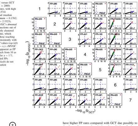
2.4.3 cMVGC performance for Model 3

Here (Fig. 18) the qualitative behaviour is the same as for the other estimators. However, as for Model 1, false deci-sion rates are out of control,—sometimes, much below GCT’s, and sometimes, way above it, irrespective of cor-rections which fail to restore Neyman–Pearson expected behaviour. Again taking GCT as reference, Fig.19shows the similarity of iPDC’s result to GCT’s with the same pattern of larger FP values well abovea=1%. The corre-sponding results for cMVGC compared with GCT portray a bias towards lower cMVGC FPs (Fig.20).

10

(

p

GCT

)

10

(

p

cMVGC

)

1

0 2 4

0 2 4 _FP=0/0

FP=7

0 2 4

0 2 4_FP=0/0

FP=17

0 2 4

0 2 4 _FP=0/0

FP=11

0 5 10 15 0

5 10 15 FN=0/0

FN=0

0 2 4

0 2 4_FP=0/0

FP=10

0 2 4

0 2 4 _FP=0/0

FP=11

0 5 10 15 0

5 10 15 FN=0/0

FN=0

2

0 2 4

0 2 4_FP=8/0

FP=7

0 2 4

0 2 4 _FP=3/0

FP=8

0 2 4

0 2 4 _FP=7/0

FP=14

0 2 4 6 8 0

2 4 6 8

FP=150/83

FP=13

0 2 4

0 2 4 _FP=7/0

FP=7

0 5 10 15 0

5 10 15 FN=0/0

FN=0

0 5 10 15 0

5 10 15 FN=0/0

FN=0

3

0 2 4

0 2 4 FP=5/1

FP=17

0 2 4

0 2 4 _FP=1/0

FP=16

0 2 4

0 2 4FP=58/25

FP=8

0 2 4

0 2 4 _FP=1/1

FP=11

0 2 4

0 2 4 _FP=14/3

FP=13

0 2 4

0 2 4 _FP=3/0

FP=12

0 5 10 15 0

5 10 15 FN=0/0

FN=0

4

0 5 10 15 0

5 10 15 FN=0/0

FN=0

0 2 4 6

FP=118/44

FP=13

0 2 4

0 2 4 _FP=6/0

FP=16

0 2 4

0 2 4 _FP=29/7

FP=9

0 2 4

0 2 4 _FP=7/2

FP=9

0 2 4

0 2 4_FP=10/0

FP=10

0 5 10 15 0

5 10 15 FN=0/0

FN=0

5

0 2 4 6 0

2 4

6FP=157/71

FP=9

0 2 4

0 2 4 _FP=11/2

FP=12

0 2 4

0 2 4 _FP=0/0

FP=20

0 2 4

0 2 4 _FP=0/0

FP=10

0 2 4

0 2 4_FP=0/0

FP=9

0 2 4

0 2 4 _FP=0/0

FP=9

0 2 4

0 2 4 _FP=0/0

FP=3

6

0 2 4

0 2 4 _FP=0/0

FP=6

0 2 4

0 2 4 FP=23/6

FP=14

0 2 4

0 2 4 _FP=5/2

FP=11

0 2 4

0 2 4_FP=6/2

FP=8

0 2 4

0 2 4 FP=6/1

FP=12

0 2 4

0 2 4 _FP=6/1

FP=9

0 5 10 15 0

5 10 15 FN=0/0

FN=0

7

Fig. 8 cMVGC versus GCT

performance (K=2000) clusters along lines, with high

b¼0:83290:5741 coefficient spread (median ¼0:8417; minimum¼0:1762; and maximum¼2:3323), confirmingcMVGC’s abnomal behaviour. Connections out of

x6 are consistently clustered

above the 45°line, which contrasts with those reaching thex1andx6consistently with

lowcMVGC FP values (top left) (except forx5!x1).cMVGC

abnormality is apparent as FP values differ much from 10 as should happen fora¼1%.

cMVGC-corrected FPs (separated by slash) do not improve the situation

3 2

1 4 5

Fig. 9 Diagram depicting the essential elements of Model 2

(9)

3 Discussion

This study presents simulation evidence about the perfor-mances of statistical connectivity tests: two in time domain and using two new frequency domain measures.

One should remind the reader that the frequency domain tests, iDTF and iPDC, measure different aspects of con-nectivity and are not immediately comparable as discussed at length in [17,18]. This contrasts with GCT,iPDC and

cMVGC which are geared towards describing the same aspect of connectivity between adjacent structures [17].

Among the tests in the latter class, GCT proved to be the one most in accord with the expected Neyman–Pearson behaviour in the sense that observed FP rates are in accord with the preset value of a justifying its employment as reference in the trial-by-trial comparisons between meth-ods as summed up herein.

QualitativelyiPDC closely mirrors GCT behaviour, and predictably produces higher FP rates as a consequence of howiPDC connectivity was detected by deeming just one frequency above threshold as significant. Whereas one may conceivably improve on how to employiPDC for testing,

10

(

p GCT

)

5

0

5 10 15

0 2 4

0 2 4 6

100 200 50010002000

0 5 10 15

4

0

2 4

0 2 4 6

0 5 10 15

0 2 4

0 2 4 6

3

0

5 10

0 5 10 15

0 2 4

2

0

5 10 15

0 2 4

0 2 4 6

1

Fig. 10 GCT performance for

Model 2 and K={100, 200, 500, 1000, 2000} data record lengths

10

(

p iPDC

)

5

0

5 10 15

0 2 4

0 2 4 6

100 200 50010002000

0 5 10 15

4

0

2 4 6

0 2 4 6

0 5 10 15

0 2 4 6

0 2 4 6 8

3

0

5 10

0 5 10 15

0 2 4

2

0

5 10 15

0 2 4 6

0 2 4

0 1 2 3 4

0 2 4 6

1

Fig. 11 iPDC performance for

(10)

its use is recommended when there is frequency content of physiological interest.

Added for comparison,cMVGC detection proved to be biased towards a reduction of the FP rates in many cases. By contrast, examination of its behaviour for other K

(available in more detail from our Web site) suggests that,

for small K, it tends to miss existing connections more often than the other methods.

Perhaps more striking and more important, however, in the sense of Neyman–Pearson detection foracompliance, is that procedures are usually constructed to impart control over FP decisions, which according to the present

10

(

p

cMVGC

)

5

0

5 10 15

0 2 4

0 5 10

100 200 50010002000

0 5 10 15

4

0

2 4

0 2 4

0 5 10 15

0 2 4

3

0

2 4 6

0 5 10 15

0 2 4

2

0

5 10 15

0 2 4

1

Fig. 12 cMVGC performance

for Model 2 and K={100, 200, 500, 1000, 2000} data record lengths

10

(

pGCT

)

10

(

p iPDC

)

1

0 2 4

0 2 4 _FP=45

FP=9

0 2 4

0 2 4 _FP=32

FP=6

0 2 4

0 2 4 FP=43

FP=20

0 2 4

0 2 4 _FP=35

FP=12

0 5 10 15

0 5 10

15 FN=0

FN=0

2

0 2 4

0 2 4 _FP=48

FP=13

0 2 4

0 2 4 _FP=28

FP=7

0 2 4

0 2 4 FP=56

FP=16

0 5 10 15

0 5 10

15 FN=0

FN=0

0 2 4

0 2 4 _FP=38

FP=17

3

0 2 4

0 2 4 _FP=41

FP=19

0 2 4

0 2 4 FP=40

FP=11

0 5 10 15

0 5 10

15 FN=0

FN=0

0 2 4

0 2 4 _FP=29

FP=5

0 2 4

0 2 4 FP=36

FP=13

4

0 5 10 15

0 5 10

15 FN=0

FN=0

0 2 4

0 2 4 FP=37

FP=13

0 2 4

0 2 4 _FP=27

FP=9

0 2 4

0 2 4 _FP=34

FP=10

0 5 10 15

0 5 10

15 FN=0

FN=0

5

Fig. 13 Comparative

performance between GCT and

iPDC detection performances at

(11)

observations, is a condition that fails to be met by the

cMVGC implementation from [9] which was used here without modification. It is also important to note that em-ploying author-recommended decision corrections [9] usually aggravates matters. It is this lack of compliance to Neyman–Pearson criteria that we termed anomalous.

Whether this happens due to an eventual software glitch, or reflects a more fundamental issue, is unknown. One should note that on many instances,cMVGC produced fewer FPs, something good in itself. This apparent quality is coun-terbalanced by much worse performance for some links, as in Model 1, in sharp contrast to other methods whose re-sults attain the prescribed a and are balanced for all con-nections to within the attainable accuracies of the Monte Carlo simulations.

Based on its good asymptotic control of FP observa-tions, it is fair to suggest that, at least provisionally, GCT, as proposed by [2], be taken as a gold standard for de-tecting connectivity between adjacent structures and that

iPDC and cMVGC should be used taking into account adequate forewarning of their present observed limitations. The present Monte Carlo simulations showed good large sample fit and robustness for Models 1 and 2. In the presence of large exogenous/latent variables (Model 3), we observed poor performance for large samples possibly due to the poor performance of the MAR model estimation algorithms under low signal-to-noise ratio regardless of the statistical procedure (K[5000). In this regard, Model 3 deserves the special comment that its comparatively worse performance is not surprising since, strictly speaking, it violates the usual assumptions behind the development of all the test detection procedures discussed herein.

10

(

pGCT

)

10

(

p c

MVGC

)

1

0 2 4

FP=5/0

FP=9

0 2 4

FP=4/1

FP=6

0 2 4

FP=7/1

FP=20

0 2 4

FP=6/0

FP=12

0 5 10 15

0 5 10 15 FN=0/0

FN=0

2

0 2 4

FP=9/3

FP=13

0 2 4

FP=2/0

FP=7

0 2 4

0 2 4 _FP=13/1

FP=16

0 5 10 15

0 5 10 15 FN=0/0

FN=0

0 2 4

0 2 4 _FP=7/2

FP=17

3

0 2 4

0 2 4 _FP=4/0

FP=19

0 2 4

0 2 4 FP=6/1

FP=11

0 5 10 15

0 5 10 15 FN=0/0

FN=0

0 2 4

0 2 4 _FP=2/1

FP=5

0 2 4

0 2 4 _FP=7/4

FP=13

4

0 5 10 15

0 5 10 15 FN=0/0

FN=0

0 2 4

0 2 4 _FP=10/3

FP=13

0 2 4

0 2 4 _FP=4/1

FP=9

0 2 4

0 2 4 _FP=5/4

FP=10

0 5 10 15

0 5 10 15 FN=0/0

FN=0

5

Fig. 14 Comparative

cMVGC detection performances at K=2000 time samples for Model 2

3 2

5 1

e6

a1

a2

a4

a5

a3

4

e z-1

z-1

+

ci bi

Exogenous common

input

Latent variable

Fig. 15 Diagram depicting the essential elements of model

intro-duced by [19] modified from Model 2 [6]. For each simulation, the parametersai were chosen randomly from a uniform distribution in

½0 1 interval, and allbi¼2 and ci¼5, while the innovations, ei,

(12)

Finally, we propose that the present methodology rep-resents the seed of a potential tool for systematically comparing connectivity estimators. The reason for this is twofold: (a) the framework provides a standardized ap-proach whereby comparisons can be made systematically and (b) may be used even in the absence of formally

rigorous statistical criteria, i.e. even if only ad hoc decision rules are available and is therefore not restricted to methods with theoretically well-established detection criteria. We have future plans to include bootstrap-based connectivity detection schemes under the same standardized framework for comparison purposes.

10

(

p GCT

)

1

0 2 4 6 8

0 5 10

0 5 10 15

2

0 2 4 6 8

0 5 10

0 5 10 15

0 2 4 6 8

3

0 5 10

0 5 10 15

0 2 4 6 8

0 5 10

4

0 5 10 15

100200500100020005000₁₀₀₀₀

0 2 4 6 8

0 5 10 15

5

Fig. 16 GCT performance on

Model 3 and K={100, 200, 500, 1000, 2000, 5000, 10000} data record lengths

10

(

p i

PDC

)

1

0 5 10

0 5 10 15

2

0 5 10

0 5 10 15

0 5 10

3

0 5 10

0 5 10 15

0 5 10

4

0 5 10 15

100200500100020005000₁₀₀₀₀

0 5 10

0 5 10 15

5

Fig. 17 iPDC performance on

(13)

10

(

p cMVGC

)

1

0 2 4 6 8

0 5 10

0 5 10 15

2

0 2 4 6 8

0 5 10

0 5 10 15

0 2 4 6 8

3

0 5 10

0 5 10 15

0 2 4 6 8

0 5 10

4

0 5 10 15

100200500100020005000₁₀₀₀₀

0 2 4 6 8

0 5 10

0 5 10 15

5

Fig. 18 cMVGC performance

on Model 3 andK={100, 200, 500, 1000, 2000, 5000, 10000} data record lengths

10

(

pGCT

)

10

(

p iPDC

)

5

0 5 10

0 5 10FN=200

FN=351

0 2 4 6

FP=120

FP=60

0 2 4 6

0 2 4 6 FP=122

FP=47

0 5 10 15

0 5 10 15 FP=143

FP=63

0 5 10 15

0 5 10 15

FN=83

FN=106

4

0 2 4 6

FP=121

FP=58

0 2 4 6

0 2 4 6 FP=112

FP=43

0 5 10 15

0 5 10

15 FN=0

FN=0

0 2 4 6

0 2 4 6 FP=132

FP=59

0 2 4 6

FP=102

FP=44

3

0 2 4 6

0 2 4 6 FP=118

FP=52

0 5 10 15

0 5 10 15 FN=41

FN=100

0 2 4

FP=124

FP=56

0 2 4

0 2 4 FP=91

FP=46

0 2 4

0 2 4 FP=107

FP=53

2

0 5 10 15

0 5 10

15 FN=0

FN=0

0 2 4 6

FP=126

FP=60

0 2 4

0 2 4 FP=105

FP=37

0 2 4

0 2 4 FP=123

FP=56

0 2 4 6

0 2 4 6 FP=109

FP=49

1

Fig. 19 Comparative

iPDC detection performances at

(14)

Acknowledgments CNPq Grant 307163/2013-0 to L.A.B. and CNPq 309381/2012-6 and FAPESP 2014/12907-3 Grants to K.S. are also gratefully acknowledged, and the authors offer thanks to NAPNA - Nu´cleo de Neurocieˆncia Aplicada from the University of Sa˜o Paulo. Part of this work was carried out during FAPESP Grant 2005/56464-9 (CInAPCe).

Open Access This article is distributed under the terms of the

Creative Commons Attribution 4.0 International License (http:// creativecommons.org/licenses/by/4.0/), which permits unrestricted use, distribution, and reproduction in any medium, provided you give appropriate credit to the original author(s) and the source, provide a link to the Creative Commons license, and indicate if changes were made.

References

1. Baccala´ LA, Sameshima K (2014) Brain connectivity. In: Sameshima K, Baccala´ LA (eds) Methods in brain connectivity inference through multivariate time series analysis. CRC Press, Boca Raton, pp 1–9

2. Lu¨tkepohl H (2005) New introduction to multiple time series analysis. Springer, New York

3. Baccala´ L, De Brito C, Takahashi D, Sameshima K (2013) Unified asymptotic theory for all partial directed coherence forms. Philos Trans R Soc A 371:1–13

4. Baccala´ LA, Takahashi DY, Sameshima K (2015) Consolidating a link centered neural connectivity framework with directed transfer function asymptotic. arXiv: q-bio.nc/1166340

5. Takahashi D, Baccala´ L, Sameshima K (2010) Information theoretic interpretation of frequency domain connectivity measures. Biol Cybern 103:463–469

6. Baccala´ LA, Sameshima K (2001) Partial directed coherence: a new concept in neural structure determination. Biol Cybern 84:463–474

7. Kamin´ski M, Blinowska KJ (1991) A new method of the de-scription of the information flow in brain structures. Biol Cybern 65:203–210

8. Sameshima K, Takahashi DY, Baccala´ LA (2014) On the sta-tistical performance of connectivity estimators in the frequency domain. In: Slezak D, Tan AH, Peters JF, Schwabe L (eds) Lecture Notes in Computer Science. Springer, Heidelberg, pp 412–423

9. Barnett L, Seth AK (2014) The MVGC multivariate Granger causality toolbox: a new approach to Granger-causal inference. J Neurosci Methods 223:50–68

10. Haufe S, Nikulin VV, Mu¨ller KR, Nolte G (2013) A critical assessment of connectivity measures for EEG data: a simulation study. NeuroImage 64:120–133

11. Wu MH, Frye RE, Zouridakis G (2011) A comparison of mul-tivariate causality based measures of effective connectivity. Comput Biol Med 41:1132–1141

12. Florin E, Gross J, Pfeifer J, Fink GR, Timmermann L (2011) Reliability of multivariate causality measures for neural data. J Neurosci Methods 198:344–358

13. Fasoula A, Attal Y, Schwartz D (2013) Comparative performance evaluation of data-driven causality measures applied to brain networks. J Neurosci Methods 215:170–189

14. Astolfi L, Cincotti F, Mattia D, Marciani MG, de Baccala LA, Vico Fallani F, Salinari S, Ursino M, Zavaglia M, Ding L, Edgar JC, Miller GA, He B, Babiloni F (2007) Comparison of different

10

(

pGCT

)

10

(

p cMVGC

)

5

0 5 10

0 5

10 _FN=480/673

FN=351

0 2 4

0 2 4 FP=22/7

FP=60

0 2 4 6

0 2 4 6 FP=14/9

FP=47

0 5 10 15

0 5 10 15 FP=26/9

FP=63

0 5 10 15

0 5 10 15

FN=141/279

FN=106

4

0 2 4 6

FP=28/10

FP=58

0 2 4 6

0 2 4 6 FP=14/7

FP=43

0 5 10 15

0 5 10 15 FN=0/0

FN=0

0 2 4

0 2

4 FP=28/16

FP=59

0 2 4

0 2 4 FP=13/5

FP=44

3

0 2 4 6

0 2 4 6 FP=15/6

FP=52

0 5 10 15

0 5 10

15 FN=210/402

FN=100

0 2 4

0 2

4 FP=32/17

FP=56

0 2 4

0 2 4 _FP=12/4

FP=46

0 2 4

0 2 4 FP=21/7

FP=53

2

0 5 10 15

0 5 10 15 FN=0/0

FN=0

0 2 4

0 2

4 FP=31/17

FP=60

0 2 4

0 2 4 FP=13/5

FP=37

0 2 4

0 2 4 FP=21/6

FP=56

0 2 4 6

0 2 4 6 _FP=15/8

FP=49

1

Fig. 20 Comparative

(15)

cortical connectivity estimators for high-resolution EEG record-ings. Hum Brain Mapp 28:143–157

15. Marple SL Jr (1987) Digital spectral analysis: with applications. Prentice Hall, Englewood Cliffs

16. Baccala´ LA, Sameshima K (2001) Overcoming the limitations of correlation analysis for many simultaneously processed neural structures. Prog Brain Res Adv Neural Popul Coding 130:33–47 17. Baccala´ LA, Sameshima K (2014) Causality and Influentiability: The need for distinct neural connectivity concepts. In: Slezak D, Tan AH, Peters JF, Schwabe L (eds) Lecture Notes in Computer Science. Springer, Heidelberg, pp 424–435

18. Baccala´ LA, Sameshima K (2014) Multivariate time series brain connectivity: a sum up. In: Sameshima K, Baccala´ LA (eds) Methods in brain connectivity inference through multi-variate time series analysis. CRC Press, Boca Raton, pp 245–251 19. Guo S, Wu J, Ding M, Feng J (2008) Uncovering interactions in

the frequency domain. PLoS Comput Biol 4:e1000087

Koichi Sameshimais a graduate in Electrical Engineering and M.D.

from the University of Sa˜o Paulo. He was trained in cognitive neuroscience, brain electrophysiology, and multivariate time series analysis at the University of Sa˜o Paulo and the University of California at San Francisco. His research interests centre around the studies of neural plasticity, cognitive function, and information pro-cessing aspects of mammalian brain through behavioural, electro-physiological, and computational neuroscience protocols. To functionally characterize collective multichannel neural activity and correlate to animal or human behaviour, normal and pathological, he

has also been seeking and developing robust and clinically useful methods and measures for brain dynamics staging, brain connectivity inferences, etc.

Daniel Y. Takahashi holds the B.Sc. degree in Applied and

Computational Mathematics (at the University of Saõ Pulo), an M.D. (the University of Saõ Paulo), and a Ph.D. in Bioinformatics (at the University of Saõ Paulo). His main interest is to better understand how animal behaviours emerge from the interaction between brain, body, environment, and other animals. To achieve such understand-ing, he has been working on developing new methods for statistical inference of dynamic interactions and on developing new animal models of social vocal communication.

Luiz A. Baccala´after majoring in Electrical Engineering and Physics

http://www.lcs.poli.usp.br/*