R E G U L A R A R T I C L E
Open Access
Identifying the most influential roads based
on traffic correlation networks
Shengmin Guo
1,2, Dong Zhou
3,4*, Jingfang Fan
5,6, Qingfeng Tong
3,4, Tongyu Zhu
1, Weifeng Lv
1,
Daqing Li
3,4and Shlomo Havlin
6*Correspondence: [email protected]
3School of Reliability and Systems
Engineering, Beihang University, Beijing, China
4National Key Laboratory of Science and Technology on Reliability and Environmental Engineering, Beijing, China
Full list of author information is available at the end of the article
Abstract
Prediction of traffic congestion is one of the core issues in the realization of smart traffic. Accurate prediction depends on understanding of interactions and
correlations between different city locations. While many methods merely consider the spatio-temporal correlation between two locations, here we propose a new approach of capturing the correlation network in a city based on realtime traffic data. We use the weighted degree and the impact distance as the two major measures to identify the most influential locations. A road segment with larger weighted degree or larger impact distance suggests that its traffic flow can strongly influence neighboring road sections driven by the congestion propagation. Using these indices, we find that the statistical properties of the identified correlation network is stable in different time periods during a day, including morning rush hours, evening rush hours, and the afternoon normal time respectively. Our work provides a new framework for assessing interactions between different local traffic flows. The captured correlation network between different locations might facilitate future studies on predicting and controlling the traffic flows.
Keywords: Traffic correlation network; Congestion propagation; Node importance
1 Introduction
Urban traffic system is among the most important critical infrastructures in modern cities. In large cities, people are experiencing traffic congestions frequently, which strongly im-pacts the efficiency and other wellfares of the commuters. Large congestions are the results of flow interaction between different sites in road networks [1]. Therefore, it is a critical and urgent issue to identify the critical road sections with large influence on others.
In fact, previous studies have proposed different methods to capture the critical road sections in different types of transportation networks. Many studies considered assessing road criticality and system reliability using system-based approaches [2–12]. For exam-ple, Jenelius et al. quantified the road importance in northern Sweden by considering the increase in a generalized travel cost, and the unsatisfied demand, as measurements of the impact of each road’s failure [3]. Another importance measurement based on the recipro-cals of the travel costs was developed by Nagurney and Qiang [4,5]. Balijepalli and Oppong compared some widely-used vulnerability indices on urban road networks, and proposed a new measurement of road criticality that is more appropriate for urban areas [6]. On
the other hand, many researchers focused in recent years on topological approaches from graph theory and network science [13–27]. For example, Demšar et al. studied the road network of Helsinki, Finland, and suggested that the cut links and links with high between-ness values tend to be the critical roads in the network [15]. Li et al. also considered the percolation process on Beijing road dynamic network, and identified bottleneck roads that play a critical role in connecting different functional clusters [21,22,27].
The above approaches have been proposed to assess the criticality of road links on the reliability and resilience [28] of road networks. To understand the critical effect on traffic reliability, it is essential to further explore the hidden dependency relation between dif-ferent components of traffic system. In fact, dependency relations are known to exist in many types of realistic systems, such as financial [29–33], climate [34–42], and biologi-cal systems [43–48], which can be captured by the correlation network approaches with similarity measures like correlation coefficients. Dependencies within and between crit-ical infrastructure systems, such as communication networks, transportation networks, and power grid, have also been explored, since they can result in cascading failures across different networks [49–53]. Therefore, the strength and range of dependency relations (or failure correlations) of each road section in the transportation network can be regarded as an important measure representing road criticality.
In this work, we investigate the road criticality in urban traffic by identifying correla-tion networks. This approach could help to capture the road seccorrela-tions that are important in understanding and predicting traffic flow propagation. We consider road velocity data with one minute resolution for each road within the 4th Ring of Beijing. In this study, we focus on 3 time periods of 5 weekdays in 2015: Rush Hour 1 (RH1, 6:30–9:30), Nor-mal Time 1 (NT1, 13:00–16:00), and Rush Hour 2 (RH2, 17:00–20:00). For each time pe-riod, we combine the 3-hour records from the 5 days, and then we remove the linear and daily trends from each record (see Methods). For each pair of road sections (here called “nodes”), we use the normalized maximal cross-correlation as the measure of link strength (link weight) [34]. To identify significant links, we compare the link weights with tempo-rally reshuffled records. In this way, the significant correlations between the records can be identifid (for more details, see Methods). Here, we only track those links with significantly larger link weights than the shuffled case.
2 Datasets and methods 2.1 Datasets
In this work, we use the velocity data in Beijing, China. The traffic dataset is recorded from floating cars in the directed road network of Beijing. Altogether, there are over 27,000 intersections and 52,000 road sections within the 5th Ring Road of Beijing. The velocity data covers real-time speed records of roads for each day with resolution of 1 minute.
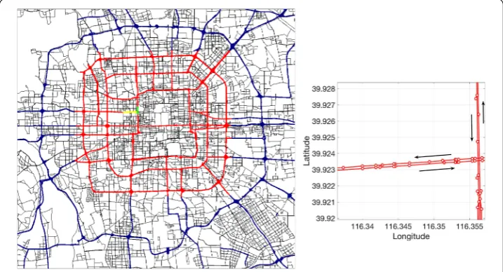
We mainly focus on the major road sections within the 4th Ring Roads. In the dataset, the road grades are classified as integers from 0 to 6. Here, level “0” means unclassified road sections; the integers from “1” to “6” are used for intercity highways, city express-ways, arterial roads, minor arterial roads, branch express-ways, and other roads, respectively. We only consider road sections with levels “1” to “3”, in order to reduce the computational complexity. In this way, we mainly focus on traffic flow and congestion propagations in the major roads of Beijing. All theN= 4530 considered road sections (also called “nodes”) within the 4th Ring Roads are shown in Fig.1(red lines). Note that each road section has its direction, from a starting point to an end point. In many cases, the two directions on the same road correspond to different road sections, as seen in Fig.1. All the road sec-tions in both direcsec-tions in a local region with two major roads (“Fuchengmen Outer St.” and “W. 2nd Ring Rd.”) can be seen in the right panel of Fig.1, and the directions of the road sections (nodes) are marked by black arrows. Each of the selectedNroad sections has a time series of measured velocity (in km·h–1) of each minute. We consider the data
of 5 weekdays: 26–30, Oct. 2015.
Note that the dataset includes missing data caused by data scarcity at some time points. To deal with this issue, we apply the following approach of interpolation: for each road section with no available data at a certain time, its velocity is defined as the average over all of its neighboring road sections, having the same direction, at that time. By repeating this procedure, we can finally obtain a complete velocity data. In fact, only a small fraction of time series need to be supplemented in the three considered time periods. For example,
in each 5-min time window in RH1 of 26, Oct. 2015, the fraction of road sections without any data in the 5 minutes is from 0.13 to 0.23.
Based on the obtained complete velocity data, we select the following three periods of time.
Rush Hour 1 (RH1): The morning rush hour from 6:30 to 9:30.
Normal Time 1 (NT1): The normal time from 13:00 to 16:00.
Rush Hour 2 (RH2): The evening rush hour from 17:00 to 20:00.
For each of these three periods, we collect the corresponding 3-hour time series (with length 180 minutes) from each of the 5 weekdays, and we combine them into one time series with total length,L= 180×5 = 900 (minutes). We denote these records asS˜∗i(t), wherei= 1, . . .Nandt= 1, . . . ,L.
2.2 Methods
2.2.1 Data preprocessing
In order to identify the correlation network from the velocity records prepared in the pre-vious subsection, we need to remove the linear and the daily trends from the time series of each node (road section), since they may produce biased correlations. For example, if both time series include similar daily periodic behavior, or they have strong linear trends (rep-resenting possible spurious effects due to the increase of traffic demand and other factors), their correlation can be very large, which is artifact and should be avoided. To eliminate the impact of these trends, we first perform a linear regression for each time seriesS˜∗i(t) (i= 1, 2, . . . ,N), and obtain its linear trend,ait+bi,t= 1, 2, . . . ,L. Then the linear trend
is removed bySi˜(t) =S˜∗i(t) – (ait+bi). Next, we remove the daily trends in the following way. We denote the time series of each nodeiafter removing the linear trend asS˜d
i(m),
whered= 1, . . . ,D= 5 andm= 1, . . . , 180 represent the considered 5 days and 180 minutes of each day, respectively. Then we calculate each minute’s mean and standard deviation by MEANi(m) =
D
d=1S˜di(m)/D, and SDi(m) =
1
D–1
D
d=1(S˜di(m) – MEANi(m))2,
respec-tively. Finally, the daily trend of each time series is removed bySid(m) =S˜
d
i(m)–MEANi(m)
SDi(m) .
We rewrite the filtered time series asSi(t),i= 1, . . . ,N,t= 1, . . . ,L. We will use this new dataset to construct traffic correlation networks.
2.2.2 Traffic correlation network inference
In order to capture the interactions between road sections with consideration of time lags, here we apply a network inference approach based on cross-correlation. The detailed pro-cedure of constructing traffic correlation networks is as follows.
For each pair of nodes (road sections)iandj, we calculate the cross-correlation function
Xi,j(τ) between the two time series,Si(t) andSj(t), whereτ= –τmax, . . . ,τmaxrepresents the
time lag. Here, forτ≥0,Xi,j(τ) is defined by
Xi,j(τ) =
L–τ
t=1(Si(t) –Si¯)(Sj(t+τ) –Sj¯)
L–τ
t=1(Si(t) –S¯i)2· L–τ
t=1(Sj(t+τ) –S¯j)2
, (1)
whereSi¯ andSj¯ are the average ofSi(t) andSj(t+τ) over the time periodt= 1, . . . ,L–τ. And forτ< 0,Xi,j(τ) =Xj,i(–τ). We useτmax= 150 (minutes) in this work. Regarding the choice
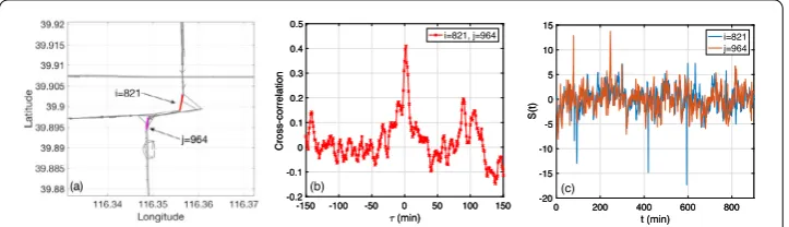
Figure 2Demonstration of a typical strong link. During the dates 26–30 Oct. 2015 in RH1. The two road sections (nodes) arei= 821,j= 964 (See (a)), withWipos,j = 4.47. (a) The location of the two nodes on the map.
The red and the magenta lines indicate the two road sectionsiandj. (b) Cross-correlationXi,j(τ) VSτ. The
maximum correlation is 0.4102, at time lagτ= 2 (minutes). (c) Shifted time series for the example in (a,b). For this link, the peak of the cross-correlation function atτ= 2 (minutes) suggests an influence with a clear direction fromitoj
cross-correlation, while it cannot be too large, since the minimal length of remaining time series for calculating correlation will be onlyL–τmax. We have also tested that choosing
τmax= 100 orτmax= 200 will not strongly impact our results, as shown in Fig. S8 in the
Additional file1. One example of the cross-correlation function and the two time series can be seen in Fig.2(b), (c). Figure2(a) shows the location of these two nodes using red and magenta lines. These two road sections are close to each other, and are in the same direction. They are found to have a maximal correlation larger than 0.4 at time lagτ= 2 minutes.
For all pairs of nodes (road sections), we define the positive link weight as Wipos,j =
max(Xi,j(τ))–mean(Xi,j(τ))
std(Xi,j(τ)) , and the time delay of this link, τ
pos
i,j , is defined as the value of τ
where the cross-correlation function Xi,j(τ) reaches its maximum. Here max(Xi,j(τ)),
mean(Xi,j(τ)) and std(Xi,j(τ)) are the maximum value, mean value, and the standard
devia-tion of the cross-correladevia-tion funcdevia-tionXi,j(τ) respectively in the range ofτ= –τmax, . . . ,τmax.
Note that the definition of link weights and time delays used in this work are expected to identify the potential interactions among road sections, especially the propagation of congestion events. Here, if the peak correlation value is significantly larger than correla-tions at otherτ values,Wipos,j tends to be large; otherwise,Wipos,j will be small. Based on our experience in handling time series of complex systems, including climate and biol-ogy, correlation links with largeWipos,j can well capture the significant impacts and filter out the environmental noise. This definition of link weights reduces the impact of auto-correlations in the time series on cross-correlation. Consider that we have removed the linear and the daily trends from each time series in this work. Therefore, the obtained strong cross-correlations are expected to well reflect inherent interactions between road segments, caused by propagation of traffic congestions. In some previous works about traffic systems, correlation-based approaches have been also applied for measuring in-teractions between traffic system components [54–60]. The link illustrated in Fig.2is a typical example of strong positive links we have captured. The link weight of this link is
we can find that most of the strong links have small time delay|τipos,j | ≤2 minutes, which is rarely influenced by state comparison of different days. Therefore, these links reflect the correlations of fast interaction in the same day, and the comparison between different days can be ignored in this work.
Finally, for each two nodesiandj, we define their distanceDi,jas the smaller one of the
great circle distance between the ending point of nodeiand the starting point of node
j, and that between the ending point of nodejand the starting point of nodei. In this way, ifiandjare neighboring road sections in the same direction, their distance will be
Di,j= 0, independent of road segment lengths. Note that under this definition of distance,
sometimes two parallel road sections may have very short distance, although they are not so close along the traffic paths. However, we argue that two parallel roads could compen-sate each other in the traffic flow, which makes it reasonable to consider they are “close”. Therefore, this issue does not impact our results.
2.2.3 Shuffling procedure
In this work, we test the significance of all link weights by comparing with the surrogate (shuffled) sample. Therefore, we perform the following shuffling procedure to generate correlation networks in the surrogate case.
For each pair of nodesiandj, we randomly shuffle the two time seriesSi(t) andSj(t) independently with hourly intervals. All the 15 hours of each time series are shuffled. In this way, the variation within each hour has been kept. Then we calculate the link weight and the time delay of this link again. In this way, we finally obtain another correlation network, with the link weights and time delay values in the shuffled case.
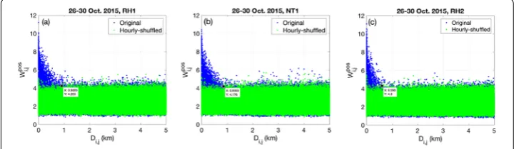
In Fig.3, we compare all the link weightsWipos,j in the original and shuffled correlation networks for the considered three time periods. For example, Fig.3(a) showsWipos,j (origi-nal and shuffled) as a function of link lengthDi,jin RH1. To make the comparison clearer,
thex-axis is limited from 0 to 5 km. We find that the original link weights exhibit larger val-ues within short distance compared to the shuffled case, where the original and the shuf-fled cases do not show significant differences for longer links. According to this, for RH1 we consider a threshold,Wmin= 4.2, for the original link weights, and another threshold,
Dmax= 0.91, for the link lengths. We only consider links withWipos,j ≥WminandDi,j≤Dmax.
All the other links are regarded as spurious links, and will be excluded from the correlation
Figure 3Thresholds for constructing correlation networks. (a)Wipos,j VSDi,j. The results after hourly shuffling
are shown by green points. Here, for each pair of nodesiandj, we randomly shuffle the two time series independently with hourly intervals. To make the comparison clearer, thex-axis is limited from 0 to 5 km. The thresholds for constructing network is thusWmin= 4.2 andDmax= 0.91 (km). (b), (c) The same as (a) but for NT1 and RH2. The corresponding thresholds areWmin= 4.2,Dmax= 0.86 (km) for NT1, andWmin= 4.3,
network. Figure3(b), (c) shows the same as Fig.3(a) but for NT1 and RH2. According to these figures, we set the thresholds for these two periods:Wmin= 4.2 andDmax= 0.86 for
NT1;Wmin= 4.3 andDmax= 0.60 for RH2. Based on these thresholds, we can obtain the
final correlation networks for RH1, NT1, and RH2, respectively.
3 Results
3.1 Weighted degree measurement
Based on the Beijing road speed records and the approach of constructing correlation networks introduced in the previous section, we can obtain a weighted network of sig-nificantly strong correlation relations. In this subsection, we use the weighted degree of nodes as a measure of road influence. Here, we consider the above mentioned thresh-oldsWminfor the link weight, andDmaxfor the link distance. Note that the calculated link
weights are impacted by the physical proximity of nodes. According to our results, most significantly strong correlation links are found to be between neighbors or the 2nd/3rd neighbors in the road networks. This reflects the nature of road networks, where the traf-fic flow on a road section tends to strongly influence its neighboring road sections first. On the other hand, strong links between neighboring nodes are a bit trivial. Therefore, we further consider only links with distanceDi,j≥0.1 kms, and the absolute time delay |τipos,j | ≤10 (minutes). In this way, we exclude the trivial links with very small link lengths and suspected links that with impacts longer than 10 minutes. This will also reduce the artificial strong correlation between neighboring nodes caused by the data compensation. After that, we calculate the weighted degree of each node as the sum of its link weights with its neighboring nodes. The definition of weighted degree includes both the number of connections and their strengths. Therefore, it can be well applied to quantify the impact of specific nodes in the urban traffic. We will capture the nodes with the largest weighted degrees, as well as the major differences between the three considered periods.
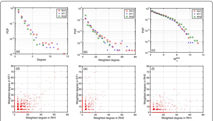
Figure4shows the distribution of weighted degrees in the considered three periods of time. First, Fig.4(a), (b) shows the distribution of degree and weighted degree values in RH1, NT1 and RH2, respectively. We find that the (weighted) degree distribution is ap-proximately exponential for different stages. The three periods of time are similar in their (weighted) degree distributions. Note, however, that RH1 and NT1 have longer tails com-pared to RH2. Figure4(c) shows the distribution of the link weightsWipos,j among the above mentioned subset of links. We find that the link weight values also exhibit exponential dis-tributions, and the decay is faster at aroundWipos,j = 8 in all three time periods. According to Fig.4(a)–(c), the statistical structure of the correlation network is quite stable over the three considered periods.
The relations between weighted degrees of nodes in different time periods are shown in Fig.4(d)–(f ). We find that a large fraction of links still have significant differences in their weighted degree during different periods, while the Pearson correlation between different periods for the whole set is not small. Later we will point out the specific subsets of nodes that are stable in different periods of time.
Figure5further shows the distribution of link lengths in RH1, NT1 and RH2. We find that the link lengths also have an approximately exponential distribution. Note that RH1 and NT1 have slightly longer links (longer than 0.6 km) compared with RH2. Therefore, roads in RH2 have shorter influence distance than RH1 and NT1.
Figure 4Statistics of weighted degree of nodes. (a) PDF of degree values at RH1 (red circles), NT1 (blue crosses), and RH2 (green squares). We consider links withWipos,j ≥Wmin,Di,j≤Dmax,Di,j≥0.1, and|τipos,j | ≤10.
(b) The same as (a) but for the weighted degrees. (c) PDF ofWipos,j of the selected links in (a), (b). (d) Weighted degree at NT1 VS at RH1. Pearson’s correlation: 0.6538. (e) Weighted degree at NT1 VS at RH2. Pearson’s correlation: 0.4874. (f) Weighted degree at RH2 VS at RH1. Pearson’s correlation: 0.4459. The data is during 26-30 Oct. 2015,N= 4530,L= 900, andτmax= 150
Figure 5PDF of strong link lengths (in km). RH1 (red circles), NT1 (blue crosses), and RH2 (green squares). The data is during 26–30 Oct. 2015, N= 4530,L= 900, andτmax= 150
Figure 6Road sections with the 20% largest weighted degrees on Beijing map. (a), (b) RH1 and NT1. 223 nodes in RH1 (green segments) and 227 nodes in NT1 (yellow segments), with 90 overlapping nodes (red segments). The percentages of the overlapping nodes among the selected hub nodes in RH1 and NT1 are 40.4% and 39.7%, respectively. (c) RH2. 116 nodes in RH2 (yellow segments), with 56 overlapping nodes with RH1 (red segments). The percentage of the overlapping nodes among the 116 selected hub nodes is 48.3%. (d) Demonstration of nodei= 750, with a large weighted degree (38.1) in RH1. The node is shown as a red segment, and its 6 links (in different colors) with other nodes. The data is during 26–30 Oct. 2015,N= 4530, L= 900, andτmax= 150
traffic (e.g. around Beijing West Station). If one hub node has a congestion event, it tends to propagate to other nodes through the identified strong correlation links.
According to these figures, only a small fraction of nodes (road sections) have very large degrees in both RH1 and NT1/RH2. The overlapping hub nodes in all the three periods include “W. 3rd Ring Rd. N. (south to north)” as well as “E. 3rd Ring Rd. Middle (north to south)”. We also illustrate an example of nodes with the 20%largest weighted degree values in RH1 in Fig.6(d) (red segment, along “W. 4th Ring Rd. Middle (north to south)”). This road section has 6 significant links with other road sections in RH1, and it has a weighted degree value of 38.1. The road sections captured here have more and stronger interactions with other nodes, and they may play the most active roles in influencing (or being influenced by) other road sections.
Figure 7Heat maps of major differences between weighted degrees in different time periods. (a) 465 nodes in RH1 with more than 4 times larger weighted degrees than NT1. The color of each node shows its weighted degree in RH1. (b) 486 nodes in NT1 with more than 4 times larger weighted degrees than RH1. The color of each node shows its weighted degree in NT1. (c) 182 nodes in RH2 with more than 4 times larger weighted degrees than NT1. (d) 752 nodes in NT1 with more than 4 times larger weighted degrees than RH2. (e) 764 nodes in RH1 with more than 4 times larger weighted degrees than RH2. (f) 210 nodes in RH2 with more than 4 times larger weighted degrees than RH1. The data is during 26–30 Oct. 2015,N= 4530,L= 900, and τmax= 150
Figure 8Relation between the mean road speed in the different time periods and weighted degrees. (a) Mean road speed (in km·h–1) over the time period VS weighted degree during RH1. Pearson’s correlation: 0.0950. (b), (c) The same as (a) but during NT1 and RH2. Pearson’s correlations: 0.0878 and 0.0182. The data is during 26–30 Oct. 2015,N= 4530,L= 900, andτmax= 150
only 182 and 210 road sections are found to have much larger weighed degrees in RH2 than in NT1 and RH1. Two examples are “Lianhuachi W. Rd.” and “Landianchang N. Rd.”. Finally, we compare the weighted degree value of each node with the average road speed of this node over the considered time period. To this end, we show in Fig.8the scatter plot of the mean speed (in km·h–1) and the weighted degree of the road. We find that in all
three considered time periods, the largest weighted degrees are surprisingly not the slow-est roads nor the fastslow-est but correspond to intermediate road speeds around 30–40 km· h–1; while the road sections with the highest or the lowest speeds have smaller weighted
degrees. Thus, the fastest and the most congested roads are not necessarily the most in-fluential. We will discuss a possible reason for this in the next subsection.
3.2 Average impact distance measurement
In this subsection, we concentrate on another property of the considered nodes (road sec-tions): the mean impact distance, defined as the average length of each node’s correlation links. Different from the impact strength, the impact distance is another critical issue in evaluating the influential range of different single nodes (road sections). Here, for each node we calculate the average link length (Di,j) over all of its selected significant links as
in the previous subsection as a measure for the impact distance.
Figure 9Statistics of the mean impact distance of nodes. (a) PDF of mean impact distance at RH1 (red circles), NT1 (blue crosses), and RH2 (green squares). (b) Mean impact distance (in km) during NT1 VS during RH1. (c) Mean impact distance during NT1 VS during RH2. (d) Mean impact distance during RH2 VS during RH1. The data is during 26–30 Oct. 2015,N= 4530,L= 900, andτmax= 150. Pearson’s correlation: (b) 0.7463, (c) 0.6926, (d) 0.6402
largest impact distances in RH1 include “N. 4th Ring Rd. W. (east to west)”, “Wanquanhe Rd. and Yuanmingyuan W. Rd. (south to north)”, “S. 4th Ring Rd. W. (west to east)”, “S. 3rd Ring Rd. W. (both directions)”, and “E. 4th Ring Rd. S. (north to south)”. In NT1, “N. 4th Ring Rd. W. (east to west)”, “Landianchang N. Rd. (north to south)”, “Lianhuachi E. Rd. (east to west)”, “S. 4th Ring Rd. W. (both directions)”, and “S12 Airport Expy (north to south)” tend to have the largest mean impact distances. Finally, in RH2, the major largest mean impact distance roads are “Lianhuachi W./E. Rd. (west to east)” and “W. 4th Ring Rd. S. (south to north)”. Similar to some hub nodes presented in the previous subsection, some of these roads correspond to locations with heavy traffic. Here, if one node with the largest mean impact distance has been congested, it tends to impact more nodes within longer range. Several typical nodes with the largest mean impact distances in all these pe-riods are “N. 4th Ring Rd. W.”, “S. 3rd Ring Rd. W.”, and “Landianchang S. Rd.”. These road sections can therefore impact (or be impacted by) more nodes within longer range during both rush hour and normal time.
In Fig. 11(a)–(c), we show the relation between the impact distance and the mean road velocity (in km · h–1) over the considered time period. Here we find that larger
Figure 10 Road sections with 20% largest mean impact distances on the map. (a), (b) During RH1 and NT1. The map shows 223 nodes in RH1 (green lines) and 227 nodes in NT1 (yellow segments), with 77 overlapping nodes (red segments). The percentages of the overlapping nodes among the selected 223 and 227 nodes in RH1 and NT1 are 34.53% and 33.92%, respectively. (c) During RH2. On the map we show 116 nodes in RH2 (yellow segments), with 32 overlapping nodes with RH1 (red segments). The percentage of the overlapping nodes among the 116 selected hub nodes is 27.59%. The data is during 26–30 Oct. 2015,N= 4530,L= 900, andτmax= 150
Figure 11 Mean road speed over the considered time period VS mean impact distance. (a) During RH1 (b) During NT1. (c) During RH2. The data is during 26–30 Oct. 2015,N= 4530,L= 900, andτmax= 150. Pearson’s correlation: (a) 0.3187, (b) 0.4103, (c) 0.1957
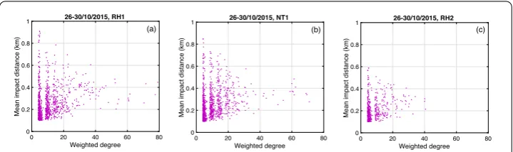
Figure 12 Mean impact distance VS weighted degree. (a) During RH1 (b) During NT1. (c) During RH2. The data is during 26–30 Oct. 2015,N= 4530,L= 900, andτmax= 150. Pearson’s correlation: (a) 0.2402, (b) 0.2226, (c) 0.2406
4 Discussion
Understanding urban traffic in large cities like Beijing is critical since congestion events frequently happen and impact the operational reliability in both the local regions and the entire system. Therefore, it is important to understand the influence of roads on other roads, i.e. how the change of traffic condition propagates. This could provide useful guid-ance for designing early warning signals for the formation of large congestions. In this direction, one important step is to reveal the existing dependency relations between dif-ferent road sections in the city, and to assess their criticality according to the captured dependencies. In principle, these dependencies are caused by propagations of traffic flow. Finding these dependencies can tell us which road sections to adjust when we wish to influence the other roads.
In this work, we developed a traffic network approach and identified the correlation net-work from realtime traffic data of Beijing traffic. We consider three time periods (morn-ing/evening rush hours and afternoon normal time) during 5 weekdays. We successfully capture the significantly strong correlations between road sections within the 4th Ring re-gion, for each considered time period. We find that the significant links usually have only lengths smaller than approximately 0.9 kms. More importantly, the road sections with the highest weighted degree or the largest mean impact distance have been identified. These most influential road sections can be related to different possible reasons, such as the den-sity of intersections, the road capacity, and the land use around the road. The effects of these factors are embedded in the correlation information we found. A road section may have a larger weighted degree, caused by its bottleneck effect. We will study these valuable issues in future works.
prediction for up to 1 hour in advance [59]. Pan et al. introduced spatio-temporal corre-lations into the stochastic cell transmission model (SCTM), and applied their model to short-term traffic state prediction [60]. In these works, e.g. in [59], spatial correlations are correlations between different nodes at a fixed time point over different days, and tempo-ral correlations are correlations between two time points for the same node over differ-ent days. Compared to these previous measures, our approach considers the correlation strength between two road sections over time, and their time lag, altogether. Specially, we explore the correlation relation as a network, and calculate some structural properties of the correlation network. Therefore, we believe that our study will help to develop new prediction methods in the future study. In summary, our findings can provide insights for better understanding complex urban transportation systems, and could facilitate future studies on predicting and controlling extreme jam propagations. The identified correla-tion network can also help to divide the city into different influential regions. Given the importance of identifying and controlling the macroscopic fundamental diagram (MFD) curves [61–64], division based on correlation networks may produce possible alternative solutions for optimizing the MFD.
Supplementary information
Supplementary informationaccompanies this paper athttps://doi.org/10.1140/epjds/s13688-019-0207-7.
Additional file 1.Supplementary information (PDF 8.1 MB)
Acknowledgements
Not applicable.
Funding
This work is supported by the National Natural Science Foundation of China (71822101, 71771009) and the Fundamental Research Funds for the Central Universities. JF and SH were supported by the Israel-Italian collaborative project NECST, Israel Science Foundation, ONR, Japan Science Foundation, BSF-NSF, and DTRA (Grant No. HDTRA-1-10-1-0014).
Abbreviations
Not applicable.
Availability of data and materials
The datasets generated and analysed during the current study are not publicly available since the authors have agreements with the data provider.
Competing interests
The authors declare that they have no competing interests.
Authors’ contributions
DL, SG, JF and SH designed the study. SG provided the data. DZ and SG performed the analyses. DZ, DL, SG, QT, TZ and WL wrote the draft of the paper. All authors helped to improve the manuscript. All authors read and approved the final manuscript.
Author details
1State Key Laboratory of Software Development Environment, Beihang University, Beijing, China.2Beijing PalmGo
Infotech Co., Ltd, Beijing, China.3School of Reliability and Systems Engineering, Beihang University, Beijing, China. 4National Key Laboratory of Science and Technology on Reliability and Environmental Engineering, Beijing, China. 5Potsdam Institute for Climate Impact Research, Potsdam, Germany.6Department of Physics, Bar-Ilan University,
Ramat-Gan, Israel.
Publisher’s Note
Springer Nature remains neutral with regard to jurisdictional claims in published maps and institutional affiliations.
References
1. Kerner BS (1999) Congested traffic flow: observations and theory. Transp Res Rec 1678:160–167.
https://doi.org/10.3141/1678-20
2. Murray-Tuite P, Mahmassani H (2004) Methodology for determining vulnerable links in a transportation network. Transp Res Rec 1882:88–96.https://doi.org/10.3141/1882-11
3. Jenelius E, Petersen T, Mattsson L-G (2006) Importance and exposure in road network vulnerability analysis. Transp Res, Part A, Policy Pract 40(7):537–560.https://doi.org/10.1016/j.tra.2005.11.003
4. Nagurney A, Qiang Q (2007) Robustness of transportation networks subject to degradable links. Europhys Lett 80(6):68001
5. Nagurney A, Qiang Q (2012) Fragile networks: identifying vulnerabilities and synergies in an uncertain age. Int Trans Oper Res 19(1–2):123–160.https://doi.org/10.1111/j.1475-3995.2010.00785.x
6. Balijepalli C, Oppong O (2014) Measuring vulnerability of road network considering the extent of serviceability of critical road links in urban areas. J Transp Geogr 39:145–155.https://doi.org/10.1016/j.jtrangeo.2014.06.025
7. Gedik R, Medal H, Rainwater C, Pohl EA, Mason SJ (2014) Vulnerability assessment and re-routing of freight trains under disruptions: a coal supply chain network application. Transp Res, Part E, Logist Transp Rev 71:45–57.
https://doi.org/10.1016/j.tre.2014.06.017
8. Rupi F, Bernardi S, Rossi G, Danesi A (2015) The evaluation of road network vulnerability in mountainous areas: a case study. Netw Spat Econ 15(2):397–411.https://doi.org/10.1007/s11067-014-9260-8
9. Wei D, Liu H, Qin Y (2015) Modeling cascade dynamics of railway networks under inclement weather. Transp Res, Part E, Logist Transp Rev 80:95–122.https://doi.org/10.1016/j.tre.2015.05.009
10. Lepri B, Antonelli F, Pianesi F, Pentland A (2015) Making big data work: smart, sustainable, and safe cities. EPJ Data Sci 4(1):16.https://doi.org/10.1140/epjds/s13688-015-0050-4
11. Bagloee SA, Sarvi M, Wolshon B, Dixit V (2017) Identifying critical disruption scenarios and a global robustness index tailored to real life road networks. Transp Res, Part E, Logist Transp Rev 98:60–81.
https://doi.org/10.1016/j.tre.2016.12.003
12. Chen L-M, Liu YE, Yang S-JS (2015) Robust supply chain strategies for recovering from unanticipated disasters. Transp Res, Part E, Logist Transp Rev 77:198–214.https://doi.org/10.1016/j.tre.2015.02.015
13. Latora V, Marchiori M (2001) Efficient behavior of small-world networks. Phys Rev Lett 87:198701.
https://doi.org/10.1103/PhysRevLett.87.198701
14. Latora V, Marchiori M (2005) Vulnerability and protection of infrastructure networks. Phys Rev E 71:015103.
https://doi.org/10.1103/PhysRevE.71.015103
15. Demšar U, Špatenkov˘a O, Virrantaus K (2008) Identifying critical locations in a spatial network with graph theory. Trans GIS 12(1):61–82.https://doi.org/10.1111/j.1467-9671.2008.01086.x
16. Youn H, Gastner MT, Jeong H (2008) Price of anarchy in transportation networks: efficiency and optimality control. Phys Rev Lett 101:128701.https://doi.org/10.1103/PhysRevLett.101.128701
17. Berche B, von Ferber C, Holovatch T, Holovatch Y (2009) Resilience of public transport networks against attacks. Eur Phys J B 71(1):125–137.https://doi.org/10.1140/epjb/e2009-00291-3
18. Woolley-Meza O, Thiemann C, Grady D, Lee JJ, Seebens H, Blasius B, Brockmann D (2011) Complexity in human transportation networks: a comparative analysis of worldwide air transportation and global cargo-ship movements. Eur Phys J B 84(4):589–600.https://doi.org/10.1140/epjb/e2011-20208-9
19. Berche B, Ferber CV, Holovatch T, Holovatch Y (2012) Transportation network stability: a case study of city transit. Adv Complex Syst 15(supp01):1250063.https://doi.org/10.1142/S0219525912500634
20. Duan Y, Lu F (2014) Robustness of city road networks at different granularities. Phys A, Stat Mech Appl 411:21–34.
https://doi.org/10.1016/j.physa.2014.05.073
21. Li D, Fu B, Wang Y, Lu G, Berezin Y, Stanley HE, Havlin S (2015) Percolation transition in dynamical traffic network with evolving critical bottlenecks. Proc Natl Acad Sci USA 112(3):669–672.https://doi.org/10.1073/pnas.1419185112
22. Wang F, Li D, Xu X, Wu R, Havlin S (2015) Percolation properties in a traffic model. Europhys Lett 112(3):38001 23. Cook A, Blom HAP, Lillo F, Mantegna RN, Miccichè S, Rivas D, Vázquez R, Zanin M (2015) Applying complexity science
to air traffic management. J Air Transp Manag 42:149–158.https://doi.org/10.1016/j.jairtraman.2014.09.011
24. Dunn S, Wilkinson SM (2016) Increasing the resilience of air traffic networks using a network graph theory approach. Transp Res, Part E, Logist Transp Rev 90:39–50.https://doi.org/10.1016/j.tre.2015.09.011
25. Calatayud A, Mangan J, Palacin R (2017) Vulnerability of international freight flows to shipping network disruptions: a multiplex network perspective. Transp Res, Part E, Logist Transp Rev 108:195–208.
https://doi.org/10.1016/j.tre.2017.10.015
26. Zhang L, Zeng G, Guo S, Li D, Gao Z (2017) Comparison of traffic reliability index with real traffic data. EPJ Data Sci 6(1):19.https://doi.org/10.1140/epjds/s13688-017-0115-7
27. Zeng G, Li D, Guo S, Gao L, Gao Z, Stanley HE, Havlin S (2019) Switch between critical percolation modes in city traffic dynamics. Proc Natl Acad Sci USA 116(1):23–28.https://doi.org/10.1073/pnas.1801545116
28. Zhang L, Zeng G, Li D, Huang H-J, Stanley HE, Havlin S (2019) Scale-free resilience of real traffic jams. Proc Natl Acad Sci USA 116(18):8673–8678.https://doi.org/10.1073/pnas.1814982116
29. Onnela J-P, Chakraborti A, Kaski K, Kertész J, Kanto A (2003) Dynamics of market correlations: taxonomy and portfolio analysis. Phys Rev E 68(5):056110.https://doi.org/10.1103/PhysRevE.68.056110
30. Mizuno T, Takayasu H, Takayasu M (2006) Correlation networks among currencies. Physica A 364:336–342.
https://doi.org/10.1016/j.physa.2005.08.079
31. Tumminello M, Aste T, Di Matteo T, Mantegna RN (2005) A tool for filtering information in complex systems. Proc Natl Acad Sci USA 102(30):10421–10426.https://doi.org/10.1073/pnas.0500298102
32. Kenett DY, Shapira Y, Madi A, Bransburg-Zabary S, Gur-Gershgoren G, Ben-Jacob E (2010) Dynamics of stock market correlations. AUCO Czech Econ Rev 4(3):330–340
33. Tumminello M, Lillo F, Mantegna RN (2010) Correlation, hierarchies, and networks in financial markets. J Econ Behav Organ 75(1):40–58.https://doi.org/10.1016/j.jebo.2010.01.004
35. Mheen M, Dijkstra HA, Gozolchiani A, den Toom M, Feng Q, Kurths J, Hernandez-Garcia E (2013) Geophys Res Lett 40(11):2714–2719.https://doi.org/10.1002/grl.50515
36. Wang Y, Gozolchiani A, Ashkenazy Y, Berezin Y, Guez O, Havlin S (2013) Phys Rev Lett 111:138501.
https://doi.org/10.1103/PhysRevLett.111.138501
37. Ludescher J, Gozolchiani A, Bogachev MI, Bunde A, Havlin S, Schellnhuber HJ (2013) Improved El Niño forecasting by cooperativity detection. Proc Natl Acad Sci USA 110(29):11742–11745.https://doi.org/10.1073/pnas.1309353110
38. Ludescher J, Gozolchiani A, Bogachev MI, Bunde A, Havlin S, Schellnhuber HJ (2014) Very early warning of next El Niño. Proc Natl Acad Sci USA 111(6):2064–2066.https://doi.org/10.1073/pnas.1323058111
39. Boers N, Bookhagen B, Barbosa HMJ, Marwan N, Kurths J, Marengo J (2014) Prediction of extreme floods in the eastern Central Andes based on a complex networks approach. Nat Commun 5:5199.
https://doi.org/10.1038/ncomms6199
40. Zhou D, Gozolchiani A, Ashkenazy Y, Havlin S (2015) Teleconnection paths via climate network direct link detection. Phys Rev Lett 115(26):268501.https://doi.org/10.1103/PhysRevLett.115.268501
41. Fan J, Meng J, Ashkenazy Y, Havlin S, Schellnhuber HJ (2017) Network analysis reveals strongly localized impacts of el niño. Proc Natl Acad Sci USA 114(29):7543–7548.https://doi.org/10.1073/pnas.1701214114
42. Fan J, Meng J, Ashkenazy Y, Havlin S, Schellnhuber HJ (2018) Climate network percolation reveals the expansion and weakening of the tropical component under global warming. Proc Natl Acad Sci USA 115(52):12128–12134.
https://doi.org/10.1073/pnas.1811068115
43. Wagner A (2002) Estimating coarse gene network structure from large-scale gene perturbation data. Genome Res 12(2):309–315.https://doi.org/10.1101/gr.193902
44. Friedman N (2004) Inferring cellular networks using probabilistic graphical models. Science 303(5659):799.
https://doi.org/10.1126/science.1094068
45. Stam CJ (2004) Functional connectivity patterns of human magnetoencephalographic recordings: a ‘small-world’ network? Neurosci Lett 355(1–2):25–28.https://doi.org/10.1016/j.neulet.2003.10.063
46. Eguíluz VM, Chialvo DR, Cecchi GA, Baliki M, Apkarian AV (2005) Scale-free brain functional networks. Phys Rev Lett 94(1):18102.https://doi.org/10.1103/PhysRevLett.94.018102
47. Hecker M, Lambeck S, Toepfer S, van Someren E, Guthke R (2009) Gene regulatory network inference: data integration in dynamic models—a review. Biosystems 96(1):86–103.https://doi.org/10.1016/j.biosystems.2008.12.004
48. Greenblatt RE, Pflieger ME, Ossadtchi AE (2012) Connectivity measures applied to human brain electrophysiological data. J Neurosci Methods 207(1):1–16.https://doi.org/10.1016/j.jneumeth.2012.02.025
49. Buldyrev SV, Parshani R, Paul G, Stanley HE, Havlin S (2010) Catastrophic cascade of failures in interdependent networks. Nature 464(7291):1025–1028.https://doi.org/10.1038/nature08932
50. Gao J, Buldyrev SV, Stanley HE, Havlin S (2012) Networks formed from interdependent networks. Nat Phys 8(1):40–48.
https://doi.org/10.1038/nphys2180
51. Brummitt CD, D’Souza RM, Leicht EA (2012) Suppressing cascades of load in interdependent networks. Proc Natl Acad Sci USA 109(12):680–689.https://doi.org/10.1073/pnas.1110586109
52. Brummitt CD, Lee K-M, Goh K-I (2012) Multiplexity-facilitated cascades in networks. Phys Rev E 85:045102.
https://doi.org/10.1103/PhysRevE.85.045102
53. Zhou D, Elmokashfi A (2017) Overload-based cascades on multiplex networks and effects of inter-similarity. PLoS ONE 12(12):1–16.https://doi.org/10.1371/journal.pone.0189624
54. Knospe W, Santen L, Schadschneider A, Schreckenberg M (2002) Single-vehicle data of highway traffic: microscopic description of traffic phases. Phys Rev E 65:056133.https://doi.org/10.1103/PhysRevE.65.056133
55. Yue Y, Yeh AG-O (2008) Spatiotemporal traffic-flow dependency and short-term traffic forecasting. Environ Plan B, Plan Des 35(5):762–771.https://doi.org/10.1068/b33090
56. de Fabritiis C, Ragona R, Valenti G (2008) Traffic estimation and prediction based on real time floating car data. In: 2008 11th international IEEE conference on intelligent transportation systems, pp 197–203.
https://doi.org/10.1109/ITSC.2008.4732534
57. Chandra SR, Al-Deek H (2008) Cross-correlation analysis and multivariate prediction of spatial time series of freeway traffic speeds. Transp Res Rec 2061(1):64–76.https://doi.org/10.3141/2061-08
58. Chandra SR, Al-Deek H (2009) Predictions of freeway traffic speeds and volumes using vector autoregressive models. J Intell Transp Syst 13(2):53–72.https://doi.org/10.1080/15472450902858368
59. Min W, Wynter L (2011) Real-time road traffic prediction with spatio-temporal correlations. Transp Res, Part C, Emerg Technol 19(4):606–616.https://doi.org/10.1016/j.trc.2010.10.002
60. Pan TL, Sumalee A, Zhong RX, Indra-payoong N (2013) Short-term traffic state prediction based on temporal–spatial correlation. IEEE Trans Intell Transp Syst 14(3):1242–1254.https://doi.org/10.1109/TITS.2013.2258916
61. Geroliminis N, Daganzo CF (2008) Existence of urban-scale macroscopic fundamental diagrams: some experimental findings. Transp Res, Part B, Methodol 42(9):759–770.https://doi.org/10.1016/j.trb.2008.02.002
62. Daganzo CF, Geroliminis N (2008) An analytical approximation for the macroscopic fundamental diagram of urban traffic. Transp Res, Part B, Methodol 42(9):771–781.https://doi.org/10.1016/j.trb.2008.06.008
63. Ji Y, Geroliminis N (2012) On the spatial partitioning of urban transportation networks. Transp Res, Part B, Methodol 46(10):1639–1656.https://doi.org/10.1016/j.trb.2012.08.005