Triangulation of Input–Output Tables Based on Mixed Integer Programs for Inter-temporal and Inter-regional Comparison of Production Structures

DOI10.1186/2193-2409-3-2

R E S E A R C H Open Access

Triangulation of Input–Output Tables Based on Mixed

Integer Programs for Inter-temporal and Inter-regional

Comparison of Production Structures

Yasushi Kondo

Received: 2 October 2013 / Accepted: 18 March 2014 / Published online: 15 April 2014

© 2014 Y. Kondo; licensee Springer. This is an Open Access article distributed under the terms of the Creative Commons Attribution License (http://creativecommons.org/licenses/by/2.0), which permits unrestricted use, distribution, and reproduction in any medium, provided the original work is properly cited.

Abstract Understanding the industrial structure of a national or regional economy is one of the central issues in economics. The triangulation of an input–output table (IOT) can be employed to understand the production structure of an economy. Inter-temporal and inter-regional comparisons of multiple IOTs have addressed interesting and important issues pertaining to international trade, economic growth, and inter-industry relationships in the economy. Rank correlation coefficients between sector rankings obtained by solving optimization problems have been utilized to quantify similarities among production structures. However, it is well known that calculated rank correlations might be weak even if underlying structures are similar because the optimization problem inherently has multiple optimal solutions, thus leading to erro-neous interpretations. This paper proposes a new method to triangulate IOTs based on mixed integer programs (MIPs) for comparing the production structures of mul-tiple economies. The proposed new method does not suffer from non-uniqueness of optimal solutions and is consistent with maximization of the Kendall rank correla-tion coefficient. The applicacorrela-tion of the proposed method to the Japanese economy demonstrates stability of the Japanese production structure during 1995–2005. Com-parisons of triangulated IOTs further reveal similarities in production structures of the Chinese, Japanese, and the U.S. economy for the year 2009.

Keywords Triangularization·Fundamental structure of production·Production structure·Mixed integer program·Input–output table

JEL Classification C61·C67·L16

Electronic supplementary materialThe online version of this article (doi:10.1186/2193-2409-3-2) contains supplementary material.

Y. Kondo (

_B

Faculty of Political Science and Economics, Waseda University, 1-6-1 Nishi-waseda, Shinjuku-ku, Tokyo, 169-8050 Japan

List of Abbreviations IOT: Input–output table MIP: Mixed integer program IP: Integer program

WIOD: World Input–Output Database

1 Introduction

The entire production structure of a national or regional economy can be represented through its input–output table (IOT), consisting of extensive numerical data on differ-ent branches of national and regional economies. Quantitative methods for summariz-ing and visualizsummariz-ing information archived in IOTs are indispensable, since understand-ing the industrial structure of an economy is one of the central issues in economics. Triangulation of IOTs is one such method that facilitates summarization and analysis of data. This paper proposes a new method to triangulate IOTs based on mixed integer programs (MIPs) for examining production structures of economies, and conducting inter-temporal and inter-regional comparisons.

Primary, secondary, and tertiary sectors in an IOT in its original form are tradi-tionally arranged in the aforementioned order. An IOT of sufficiently detailed sector classification has many zero elements and it is a sparse matrix because most sectors require product inputs from a limited number of sectors. Therefore, an IOT may be triangulated, implying that most elements in the upper triangular part are zeros, by rearranging the sectors based on degrees of fabrication. Triangulation arrangement is fairly straightforward for sectors among which relative degrees of fabrication are clearly defined based on expert knowledge of industrial technologies. For instance, the automotive sector is followed by motor vehicle parts sectors in a triangulated table because an automobile is more highly fabricated than its parts. However, the relative degrees of fabrication among some sectors may not always be clearly defined. In all such cases, an IOT can still be triangulated approximately, for example, by solving an optimization problem. The ordering of sectors in an IOT triangulated in this manner can be interpreted as a descending order of degrees of fabrication, by analogy with the relationship between the automotive sector and motor vehicle parts sectors. This paper proposes a new method of triangulation based on optimization problems.

business cycles and economic growth, reducing computational burden of solving sys-tems of linear equations, and enhancing forecasting and economic planning.

In addition to the applications summarized by Korte and Oberhofer (1970), trian-gulated IOTs lend themselves to useful analysis on at least two counts in the con-temporary context. First, graphical visualization of a triangulated IOT is useful in identifying inter-sectoral dependence. Triangulation greatly improves and enhances the readability of a graphically represented IOT and aids in obtaining the complete picture of inter-sectoral transactions with little loss of information for each transac-tion. Nakamura et al. (2011) provide an example of visualizing triangulated IOTs for analyzing inter-sectoral flows of iron and steel in passenger car production. The or-dering of sectors in triangulated IOTs can also be used to determine the positioning of sectors in a flow diagram. Nakamura et al. (2011) and Nakajima et al. (2013) have shown such drawings through the Sankey diagrams.

Second, the fundamental structure of production discussed by Simpson and Tsukui (1965), its inter-temporal stability, and inter-regional similarity need to be re-investigated. Following the pioneering studies by Chenery and Watanabe (1958), Leontief (1963), and Simpson and Tsukui (1965), a number of studies examined de-veloped and less dede-veloped economies through triangulated IOTs and provided em-pirical evidence that the production structures of these economies are quite similar to each other and fairly stable over time. Korte and Oberhofer (1970), Lamel et al. (1972), Santhanam and Patil (1972), Song (1977), Fukui (1986), Pryor (1994), and Östblom (1993,1997) are some such studies. With recent technological progress en-gendering factors such as promotion of industrial symbiosis, substitution of materials across sectors, and green product-service system, it is worth checking if these factors have caused a change in hierarchy among sectors. With this background, this pa-per proposes an extension of the triangulation problem for comparing the production structures of multiple economies.

The remainder of the paper is organized as follows. Section2formulates a tri-angulation problem according to available literature and extends it for developing a new method to compare two or more IOTs. The new method is applied for inter-temporal and inter-regional comparisons in Sect.3. Concluding remarks are outlined in Sect.4. Computer codes used for implementing the new method are provided in thesupplementary material.

2 Methods

2.1 Literature Review

ifn=5, enumerating then! =120 permutations and choosing an optimal solution may resolve the problem. However, such a brute force algorithm works only when the value of nis very small and its application is problematic even in the case of moderate number of sectors such asn=50 for whichn! ≈3.0×1064.

Several algorithms specifically designed for the triangulation problem have been developed and proposed in the literature. Simpson and Tsukui (1965), Korte and Oberhofer (1970), and Fukui (1986) proposed heuristic algorithms in which they have iterated substitutions of sectors, called ringshift permutations. However, op-timal solutions are not necessarily obtained by executing these algorithms. Algo-rithms with which optimal solutions can be found for problems of moderate size have also been developed. Haltia (1992) and Östblom (1997) proposed an algorithm without ringshift permutations. The triangulation problem is equivalent to the lin-ear ordering problem and more efficient algorithms for generating optimal solutions have been proposed in the literature on operations research (Grötschel et al.1984a; Laguna et al.1999; Mitchell and Borchers2000; Chiarini et al.2004; Pintea et al.

2009). Mitchell and Borchers (2000) have noted that an exact solution to a linear ordering problem with 250 objects or sectors can be obtained.

Because the triangulation problem can be represented as an integer program (IP) as explained in Grötschel et al. (1984a,1984b) and Chiarini et al. (2004), it can be solved, at least approximately, by a general-purpose algorithm for IPs implemented in currently available software. It can be said that most general-purpose algorithms are less efficient than special algorithms. However, general-purpose algorithms, unlike special algorithms, can be applied even when the original problem is extended or modified, for example, by adding constraints or changing the objective function. This paper utilizes an IP representation of the triangulation problem for comparing the production structures of multiple economies.

2.2 Definition and Representations of the Triangulation Problem

Let there benindustrial sectors and suppose that our target is to triangulate ann×n

matrixA=(Aij)that describes inter-dependence among sectors. We do not specify

this matrix in more detail here, and simply call it an IOT in this section. The next section outlines this aspect in greater detail. We define the set of natural numbers re-ferring tonsectors asN= {1, . . . , n}. We then denote a permutation ofnsectors by π=(π(1), . . . , π(n))and the set of all permutations of sectors byΠ. Given an arbi-trary permutationπ∈Π, letA(π)=(Aij(π))denote the IOT in which the sectors

are permuted according toπ. This is written as follows:

Aij(π)=Aπ(i)π(j ) (i, j∈N ). (1)

The triangulation problem is formulated as a combinatorial optimization problem:

maximize A(π)

subject to π∈Π, (2)

where(M)=_i>jMij for anyn×nmatrixM=(Mij), representing the sum of

elements in the lower triangular part.

An index called the degree of linearity has been used in the literature (e.g., Fukui

1986) to represent how well an IOT is triangulated. Given an IOT, the degree of linearity of a permutationπis defined as follows:

λA(π)=

i>jAij(π)

i=jAij(π)=

(A(π))

i=jAij

. (3)

The numerator is the same as the objective function of the triangulation problem de-scribed by (2). The denominator is the sum of all the off-diagonal elements. Note that a permutationπ that maximizes the objective function of the triangulation problem

(A(π)), also maximizes the degree of linearityλ(A(π)), because the denominator does not depend onπ.

Let us introduce the followingn×nmatrix of binary variables,X=(Xij):

Xij=1

π−1(i)≥π−1(j ) (i, j∈N ), (4) where 1{·}is the indicator function such that 1{P} =1 if the propositionP is true, and 1{P} =0 otherwise. Given a permutationπ,π(p)represents the sector at the

pth position andπ−1(s)represents the position at which sectors is placed, where “sector s” refers to the sth sector in the original ordering. Note that Xii =1 for

everyi∈N,Xij=1 if sectorj precedes sectoriin the permutationπ, andXij=0

otherwise. In other words,Aij is located in the lower triangular part or on the main

diagonal ofA(π)ifXij=1. The following equality thus holds:

A(π)= n

i=1

n

j=1

AijXij− n

i=1

It is known that the triangulation problem described in (2) can be represented as the following IP (deCani1969; Grötschel et al.1984a; Chiarini et al.2004):

maximize

n

i=1

n

j=1

AijXij− n

i=1

Aii

subject to Xii=1 (i∈N ),

Xij+Xj i=1 (i < j;i, j∈N ),

0≤Xij+Xj k−Xik≤1 (i < j < k;i, j, k∈N ),

Xij∈ {0,1} (i, j∈N ).

(6)

Alternatively, it can also be represented as the following IP:

maximize

n−1

i=1

n

j=i+1

(Aij−Aj i)Xij+Aj i

subject to 0≤Xij+Xj k−Xik≤1 (i < j < k;i, j, k∈N ),

Xij∈ {0,1} (i < j;i, j∈N ).

(7)

More specifically, the last representation is a{0,1}-program, which hasn(n−1)/2 binary variables andn(n−1)(n−2)/3 inequality constraints.

Given that an optimal solution is obtained for (7), the corresponding optimal per-mutationπcan then be derived by the following equation:

π−1(i)= n

j=1

Xij (i∈N ), (8)

whereXii=1 (i∈N) andXj i=1−Xij (i < j;i, j∈N).

2.3 Extension of the Triangulation Problem for Comparing Input–Output Tables

Suppose that we have IOTs for nT time periods, A(t ) =(A(t )_ij) (t ∈T), where T = {1, . . . , nT}and superscript “(t )” indicates the time period (the method

pro-posed in this section can be applied for inter-regional comparisons; however, this section focuses on inter-temporal comparisons). Suppose that we have solved IP (7) withA=A(t )for all time periods and obtained an optimal solutionX(t )_ij, the corre-sponding optimal permutationπ(t ), and the optimal valueM(t )(maximized objective

value) of the program. We propose to findnT sequences of sectors that are mutu-ally as close as possible, guaranteeing that best degrees of linearity are attained. The problem fornT =2 and T = {1,2}can be written as follows, with the concept of “difference” allowed to be ambiguous:

minimize difference betweenπ(1)andπ(2)

subject to A(t )(π(t ))

=M(t ) (t∈T ),

π(t )∈Π (t∈T ).

Let us define the difference betweenπ(1) andπ(2) as the sum of absolute

differ-ences between the elements ofX(1) andX(2), that is,n_i=−₁1n_j=i+1|X_ij(1)−X_ij(2)|. The advantage of this difference over others such as the sum of squared differences will be discussed later. We now introduce new variables,Uij, Vij (i < j;i, j∈N),

such that

Uij−Vij=X_ij(1)−X_ij(2), Uij≥0, Vij≥0(i < j;i, j∈N ). (10)

Note that|X_ij(1)−X(_ij2)| =Uij+Vij ifUijVij=0 and (10) hold for any pair ofX_ij(1)

andX_ij(2). This is a well-known technique for dealing with absolute values in the field of operations research.

By employing this technique, we make the program (9) concrete and propose the following MIP for comparing hierarchies among sectors in two IOTs:

minimize

n−1

i=1

n

j=i+1

(Uij+Vij)

subject to 0≤X(t )_ij +X(t )_{j k}−X_ik(t )≤1 (i < j < k;i, j, k∈N;t∈T ),

Uij−Vij=X(ij1)−X (2)

ij (i < j;i, j∈N ),

n−1

i=1

n

j=i+1

A(t )_ij −A(t )_{j i}X_ij(t )+A(t )_{j i}=M(t ) (t∈T ),

X(t )_ij ∈ {0,1} (i < j;i, j∈N;t∈T ),

Uij≥0, Vij≥0 (i < j;i, j∈N ).

(11)

The first and fourth constraints form the same set of constraints in (7) and correspond to the constraintsπ(t )∈Π (t∈T) in (9).X(1)=(X_ij(1))andX(2)=(X_ij(2))

consis-tently represent two permutations of sectors. The second and fifth constraints and the objective function compose the technique to minimize the difference betweenπ(1)

andπ(2), or

n−1

i=1

n

j=i+1|X

(1) ij −X

(2)

ij |. The third constraint corresponds to the

constraints(A(t )(π(t )))=M(t )(t ∈T) in (9) and guarantees that best degrees of

linearity are attained. It should be noted that the nonlinear constraintUijVij =0 is

not necessary in the program (11) in the sense that optimal solutions always satisfy the constraint because of the characteristics of its objective function.1Therefore, the linearity of the program, except for the binary constraints onX(t )_ij , is maintained.

The advantage of program (11), a specific form of the general program (9), over other forms is at least twofold. First, the objective function and constraints, except for integralities, are linear in variables. This linearity is almost a prerequisite because we

1_{Suppose thatU}

ijVij=0 for some feasible solution for (11). By lettingWij=min{Uij, Vij}and

replac-ing(Uij, Vij)with(Uij−Wij, Vij−Wij), we can construct another feasible solution which has a smaller

use a general algorithm, rather than develop specialized algorithms. Therefore, we do not specify the difference betweenπ(1) andπ(2) as a nonlinear formula such as the

sum of squared differences between rankings.

Second, MIP (11) is consistent with the Kendall rank correlation coefficient. Note that for any pair(i, j )such thati=j (i, j∈N),

X(_ij1)−X_ij(2)= ⎧ ⎪ ⎨ ⎪ ⎩

1 ifπ₍−₁1₎(i) > π₍−₁1₎(j )andπ₍−₂1₎(i) < π₍−₂₎1(j ), −1 ifπ₍−₁1₎(i) < π₍−₁1₎(j )andπ₍−₂1₎(i) > π₍−₂₎1(j ),

0 otherwise,

(12)

becauseX(t )_ij =1{π_{(t )}−1(i) > π_{(t )}−1(j )}(i=j;i, j∈N,t∈T) according to (4). Thus, the objective function of the proposed program (11), Q=_i<j|X_ij(1)−X_ij(2)| =

i<j(Uij +Vij), can be interpreted as the number of pairs (i, j ) of sectors that

disagree in the two rankings. Note also that the Kendall rank correlation coefficient betweenπ(1) andπ(2)is given byτ (π(1),π(2))=1−4Q/n(n−1)(see, for

exam-ple, Kendall and Gibbons1990, p. 5). Thus, it has been shown that the proposed MIP (11) maximizes the Kendall rank correlation coefficient between two sequences of sectors, guaranteeing that best degrees of linearity are attained. A variant of MIP (11) that is consistent with the Spearman rank correlation coefficient can also be formu-lated by specifying its objective function as the sum of squared differences between the rankings,n_i=1(π₍−₁₎1(i)−π₍−₂1₎(i))2. However, we will not employ this nonlinear formulation because a linear formulation is preferred to a nonlinear formulation for our study.

MIP (11) fornT =2 can be generalized for cases ofnT ≥3 as follows:

minimize

nT−1

s=1

nT

t=s+1

n−1

i=1

n

j=i+1

U_ij(st )+V_ij(st )

subject to 0≤X(t )_ij +X_{j k}(t )−X(t )_ik ≤1 (i < j < k;i, j, k∈N;t∈T ),

U_ij(st )−V_ij(st )=X_ij(s)−X(t )_ij (i < j;i, j∈N;s < t;s, t∈T ),

n−1

i=1

n

j=i+1

A(t )_ij −A(t )_{j i}X(t )_ij +A(t )_{j i}=M(t ) (t∈T ),

X(t )_ij ∈ {0,1} (i < j;i, j∈N;t∈T ),

U_ij(st )≥0, V_ij(st )≥0 (i < j;i, j∈N;s < t;s, t∈T ).

(13)

In this generalization, superscript “(st )” is introduced for Uij andVij to indicate

different time periods for comparison. For formulating the objective function in (13), sums of absolute differences between elements of X(s) _andX(t ) _{for all nT(nT −}

π(s) andπ(t ). Therefore, minimization in (13) is consistent with maximization of

the simple arithmetic mean of the Kendall rank correlation coefficients for all pair-wise comparisons, that is,c=(nT(nT −1)/2)−1_s<tτ (π(s),π(t )). This is one of the multivariate generalizations of the pair-wise Kendall rank correlation coefficient studied by Joe (1990, p. 21).

The following MIP should also be useful when a slight deterioration of the degree of linearity is acceptable in comparing the optimal ordering of sectors:

minimize

nT−1

s=1

nT

t=s+1

n−1

i=1

n

j=i+1

U_ij(st )+V_ij(st )

subject to 0≤X(t )_ij +X_{j k}(t )−X(t )_ik ≤1 (i < j < k;i, j, k∈N;t∈T ),

U_ij(st )−V_ij(st )=X_ij(s)−X(t )_ij (i < j;i, j∈N;s < t;s, t∈T ),

n−1

i=1

n

j=i+1

A(t )_ij −A(t )_{j i}X(t )_ij +A(t )_{j i}≥αM(t ) (t∈T ),

X(t )_ij ∈ {0,1} (i < j;i, j∈N;t∈T ),

U_ij(st )≥0, V_ij(st )≥0 (i < j;i, j∈N;s < t;s, t∈T ),

(14)

whereαis a constant such that 0< α≤1. MIPs (13) and (14) are the same, except for the difference in the third constraint. The smaller the value of α is, the more concordant optimal ordering of sectors is obtained at the cost of degrees of linearity. Note that MIP (13), by construction, is equivalent to MIP (14) whenα=1.

3 Empirical Applications

There are several possible choices for the target matrix to triangulate. For example, the flow matrixZ=(Zij), whereZij refers to the intermediate flow from sectorito

sectorj; the input coefficient matrixA=(Aij)=(Zij/xj), wherexj refers to the output of sectorj; the Leontief inverse matrixL=(I−A)−1; the output coefficient matrixB=(Bij)=(Zij/xi); and the Ghosh inverse matrixG=(I−B)−1. Although

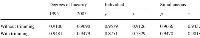
Table 1 Inter-temporal comparison of the Japanese economy between 1995 and 2005

Degrees of linearity Individual Simultaneous

1995 2005 ρ τ ρ τ

Without trimming 0.9100 0.9090 0.9579 0.9126 0.9666 0.9437 With trimming 0.9481 0.9479 0.8751 0.7329 0.9470 0.9018

Note: Rank correlation coefficients are in the columns labeled “Individual” and “Simultaneous.” “Individ-ual” refers to the results of IP (7) and “Simultaneous” refers to results of MIP (11).ρandτrefer to the Spearman and Kendall rank correlation coefficients, respectively

Source: Own calculation

Intel®Xeon®CPUs of 2.27 GHz and 24 GB RAM. The operating system and soft-ware were of 64 bits.

3.1 The Japanese Economy in 1995 and 2005: Inter-temporal Comparison

Data for the input coefficient matrices representing the production structure of the Japanese economy in 1995 and 2005 were obtained from the fixed-price tables of the Japanese Linked Input–Output Tables (SB-MIAC 2011). This particular study pe-riod is chosen because it is covered by the latest available linked IOTs. In addition to these input coefficient matrices, we also utilized “trimmed” versions of the input coefficient matrices to check the robustness of our analysis. The trimmed input coeffi-cient matrix was constructed by settingAij=0 ifAij<1/n(i, j∈N), according to

Simpson and Tsukui (1965). Typically, the larger elements are likely to be estimated more precisely, while the smaller elements possibly include more noise. The trimmed matrices are expected to emphasize significant inter-dependencies between sectors or highlight the features of production structures. The number of sectors isn=102. The number of non-zero elements of the trimmed matrix is 1104 for 1995 and 1135 for 2005, while that for the input coefficient matrix without trimming is 6321 for 1995 and 6326 for 2005. For each year, the sum of all elements of the trimmed matrix is about 84 % of the sum of all elements of the matrix without trimming, while the num-ber of non-zero elements of the trimmed matrix is considerably smaller than that of the matrix without trimming. Therefore, it can be observed that trimming effectively highlights the essential features of production structures.

Both the matrices were effectively triangulated, without trimming, by solving IP (7): the degrees of linearity were about 0.91 for each year, as shown in Table 1. The trimmed matrices were also triangulated almost perfectly and the degrees of linearity were about 0.95, as shown in Table1. These values close to unity imply that the inter-dependence among sectors can be summarized as a nearly uni-directional hierarchy. Thus, there is little multi-directional dependence such as feedback loops with substantial inter-sectoral transactions.

andτ=0.913. This result indicates that the production structure revealed by triangu-lation is fairly stable during the period 1995–2005. On the contrary, weaker correla-tion coefficients were obtained with the trimmed matrices:ρ=0.875 andτ=0.733. This result implies that either the production structure has gone through a mild change during 1995–2005 or a stable structure cannot be revealed due to non-uniqueness of optimal solutions to the triangulation problem. It is found that it is the latter in this case. Much stronger correlation such asρ=0.947 andτ =0.902 was obtained by solving MIP (11), as shown in Table1. Therefore, by utilizing the new method pro-posed in Sect.2, we could identify a fairly stable production structure in Japan during 1995–2005.

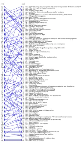
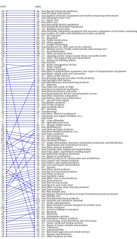
The optimal ordering of sectors obtained by solving IP (7) and MIP (11) for the trimmed matrices are shown in Figs.1and2, respectively, in the form of a migration diagram (Grötschel et al.1984b). Figure1 has much more crossings than Fig. 2. Note that the ordering of sectors in Fig.2was obtained by minimizing the number of crossings, or equivalently, by maximizing the Kendall rank correlation coefficient between orderings in 1995 and 2005, keeping the degrees of linearity equal to optimal levels. The two diagrams clearly show that a comparison based on IP (7) is strongly influenced by the non-uniqueness of optimal solutions.

As shown in Fig.2, it is found that the top 24 sectors agree with each other in the two rankings. This implies that the drastic change in hierarchies, which appears in the form of several crossings in the upper half of Fig.1, is not meaningful. The top 50 sectors approximately remain in top positions over time. Such stability in rankings is not limited to top-ranked sectors only. The difference in ranking for two years is less than 10 for 95 sectors.

Figure2shows that sector #87 “Public administration,” sector #83 “Communica-tion,” and sector #85 “Information services” drastically changed their rankings during 1995–2005. Only sector #102 “Activities not elsewhere classified” purchases the out-put of “Public administration,” and the inout-put coefficientA87,102drastically increased from 0.076 to 0.279 during 1995–2005. Thus, “Public administration” sector was lo-cated just after “Activities not elsewhere classified” sector in the 2005 rankings. It is inherently difficult to infer the economic interpretation of this result because of the highly miscellaneous nature of sector #102.

Sector #83 “Communication” and sector #85 “Information services” are located in the middle of the optimal sequence (i.e., at the 59th and 54th positions), respec-tively, in the ordering for 1995. On the contrary, these sectors are located at the bot-tom of the sequence (i.e., at the 99th and 93rd positions), respectively, in 2005. This indicates that the importance of these infrastructural service industries has gone up during 1995–2005. On an average, the input coefficients representing purchase of “Communication” and “Information services” per unit of output of industrial sectors have substantially increased by 34 % and 96 %, respectively, over the study period.

transportation, research, commerce, and finance and insurance), mining sectors, util-ity sectors (electricutil-ity), and basic products manufacturing sectors (e.g., petroleum refinery and petrochemical basic products, coal products, and metal products) are located at the bottom positions. The products of these sectors except for mining sec-tors are purchased by most industry secsec-tors, while the products of mining secsec-tors are mostly purchased by the basic products manufacturing sectors. The sectors located in the middle positions are parts manufacturing sectors (e.g., motor vehicle parts, electrical devices and parts, and semiconductor devices), light industry sectors (e.g., textile products, wooden products, and paper products), and agriculture, forestry, and fishery sectors.

This fundamental structure of the Japanese economy observed by triangulation is very similar to the fundamental structure found by Simpson and Tsukui (1965), except for the drastic changes in sector ranking mentioned above. From a point of view of empirical analysis, it is found that the fundamental structure of the Japanese economy has been fairly stable over the last decades, and it is slightly changing be-cause of the expansion of information and communication technology. From a point of view of method development, the new method for triangulation based on MIP (11) is very useful to clearly highlight exceptional difference in sector ranking between time periods.

3.2 Chinese, Japanese, and the U.S. Economies in 2009: Inter-regional Comparison

Domestic direct requirement matrices for the 2009 national input–output tables of China, Japan, and the U.S. were used for inter-regional comparison. Data were ob-tained from the World Input–Output Database (WIOD) (Timmer 2012; Dietzen-bacher et al.2013). The year 2009 is the latest available period in WIOD. The number of sectors isn=35. The number of non-zero elements is 1085 for China, 1156 for Japan, and 1148 for the U.S. These matrices are not sparse as only 6 %–11 % of 1225 elements are zero. These matrices are relatively denser than data pertaining to 102 sectors outlined in Sect.3.1 possibly because of higher aggregation of sector classification.

Although the three matrices are not sparse, they were triangulated by solving IP (7). The degrees of linearity were 0.812, 0.815, and 0.873 for China, Japan, and the U.S., respectively, as shown in Table2. These results are comparable with those re-ported in the literature. For example, Fukui (1986) showed that the degrees of linear-ity range from 0.83 to 0.94 for 22- or 29-sector IOTs of India, Italy, Japan, Korea, Norway, and the U.S. for the period 1947–1965.

Table 2 Inter-regional comparison among the Chinese, Japanese, and the U.S. economy in 2009

Country China (CHN) Japan (JPN) USA

Degrees of linearity 0.8121 0.8154 0.8732

Kendallτ

Pair of countries (CHN, JPN) (CHN, USA) (JPN, USA) Mean

Individual 0.5866 0.4622 0.6202 0.5563

Simultaneous 0.5933 0.4689 0.6202 0.5608

α=0.99 0.8857 0.8588 0.8387 0.8611

α=0.95 1.0000 1.0000 1.0000 1.0000

Note: “CHN” and “JPN” refer to China and Japan, respectively. The Kendall rank correlation coefficients are in the lower table. “Individual” refers to the results of IP (7) and “Simultaneous” refers to the results of MIP (13) or MIP (14) withα=1. The two rows at the bottom refer to the results of MIP (14) with

α=0.99 and 0.95

Source: Own calculation

MIP (14) was solved to check the possibility of further strengthening of con-cordance between ordering. The Kendall rank correlation coefficients obtained are shown in the row labeled “Simultaneous” in Table2. The result of MIP (14) with

α=1 is the same as that of MIP (13) described above. The result of MIP (14) with

α=0.99 shows that the Kendall rank correlation coefficient ranges from 0.839 to 0.886. MIP (14) withα=0.95 provides the Kendall rank correlation coefficient value equal to unity, which indicates that the optimal ordering of sectors is common to all the three countries. Therefore, the production structures of China, Japan, and the U.S. can be regarded as very similar if we accept a 5 % loss of degree of linearity.

The optimal ordering of sectors obtained by solving IP (7) and MIP (14) with

α=0.99 are shown in Figs.3and4, respectively. Note that in Fig.4, the ordering of sectors was obtained by minimizing the number of crossings drawn in the figure as well as crossings that would appear if sectors of the U.S. were connected with corresponding sectors of China. A comparison of Figs.3and4shows that production structures of the three countries appear similar on accepting a 1 % loss of degree of linearity.

Fig. 3 Sector rankings of China, Japan, and the U.S. based on individual triangulation.Note: The domestic input coefficient matrices are triangulated individually by IP (7). See also notes to Fig.1

Fig. 4 Sector rankings of China, Japan, and the U.S. based on simultaneous triangulation.Note: The domestic input coefficient matrices are triangulated simultaneously by MIP (14) withα=0.99. See also notes to Fig.1

aspects, the production structures of China, Japan, and the U.S. can be regarded as being very similar, on accepting 1 % loss of degree of linearity.

top positions, and followed by light industry sectors, basic products manufacturing sectors, utility sectors, mining sectors, and business service sectors.

4 Concluding Remarks

This paper has proposed a new method for triangulation of input–output tables (IOTs) by extending an integer-program representation of the triangulation problem for con-ducting inter-temporal and inter-regional comparisons. The new method provides se-quences of sectors that are mutually as close as possible and consistent with max-imization of the Kendall rank correlation coefficient. This study demonstrates the utility of the new method by applying it to the Chinese, Japanese, and the U.S. input– output tables. Comparisons based on individual application of the existing method for triangulation were found to be strongly influenced by the non-uniqueness of opti-mal solutions. Consequently, sopti-maller rank correlation was obtained even though the underlying production structures may be very similar. On the contrary, employment of the new method revealed similarities among the production structures of China, Japan, and the U.S. It also enabled investigation of the exceptional dissimilarity be-tween the economies by examining the sectors that were positioned differently.

Future research in this area may apply the new method to larger datasets. Ob-taining practically good solutions, instead of optimal solutions, would be useful for a large dataset because it may not be easy to solve large-scale mixed integer pro-grams on personal computers or workstations. Application of the new method to the following datasets is another important area of future research: inter-sectoral mate-rial flows (Nakamura et al.2011; Nakajima et al.2013), multi-regional input–output tables including carbon, water, and material flows embodied in trade (i.e., carbon, water, and material footprint of transacted goods and services) (Peters et al.2011; Steen-Olsen et al.2012; Wiedmann et al.2013; Tukker and Dietzenbacher2013), and standard monetary input–output tables. The application will provide a useful tool for graphically visualizing the inter-relationship among sectors from various perspec-tives.

Competing Interests

There are no conflicts of interest to declare.

Acknowledgements A preliminary version of this paper was presented at the 19th International Input– Output Conference at Alexandria, Virginia, the U.S. in June 2011. I am grateful to Dr. Richard Wood, anonymous referees, and the editor for their detailed and helpful comments. This research was partially supported by research funds from MEXT KAKENHI (24510059) and the Environment Research and Technology Development Fund (K122024) of the Ministry of the Environment, Japan.

References

Chenery HB, Watanabe T (1958) International comparisons of the structure of production. Econometrica 26(4):487–521

Chiarini BH, Chaovalitwongse W, Pardalos PM (2004) A new algorithm for the triangulation of input– output tables in economics. In: Pardalos PM (ed) Supply chain and finance. World Scientific, Singa-pore, pp 253–272 (Chap 15)

deCani JS (1969) Maximum likelihood paired comparison ranking by linear programming. Biometrika 56(3):537–545

Dietzenbacher E, Los B, Stehrer R, Timmer M, de Vries G (2013) The construction of world input–output tables in the WIOD project. Econ Syst Res 25(1):71–98

Fukui Y (1986) A more powerful method for triangularizing input–output matrices and the similarity of production structures. Econometrica 54(6):1425–1433

Grötschel M, Jünger M, Reinelt G (1984a) A cutting plane algorithm for the linear ordering problem. Oper Res 32(6):1195–1220

Grötschel M, Jünger M, Reinelt G (1984b) Optimal triangulation of large real world input–output matrices. Stat Hefte 25(1):261–295

Haltia O (1992) A triangularization algorithm without ringshift permutation. Econ Syst Res 3(3):223–234 Joe H (1990) Multivariate concordance. J Multivar Anal 35(1):12–30

Karp RM (1972) Reducibility among combinatorial problems. In: Miller RE, Thatcher JW, Bohlinger JD (eds) Complexity of computer computations. Springer, New York, pp 85–103

Kendall M, Gibbons JD (1990) Rank correlation methods, 5th edn. Edward Arnold, London

Korte B, Oberhofer W (1970) Triangularizing input–output matrices and the structure of production. Eur Econ Rev 1(4):482–511

Laguna M, Marti R, Campos V (1999) Intensification and diversification with elite tabu search solutions for the linear ordering problem. Comput Oper Res 26(12):1217–1230

Lamel J, Richter J, Teufelsbauer W (1972) Patterns of industrial structure and economic development: triangulation of input–output tables of ECE countries. Eur Econ Rev 3(1):47–63

Leontief W (1953) The input–output approach in economic analysis. In: The Netherlands Economic Insti-tute (ed) Input–output relations: proceedings of a conference on inter-industrial relations, Driebergen, Holland, pp 1–23

Leontief W (1963) The structure of development. Sci Am 209(3):148–166

Mitchell JE, Borchers B (2000) Solving linear ordering problems with a combined interior point/simplex cutting plane algorithm. In: Frenk HL, Roos C, Terlaky T, Zhang S (eds) High performance optimiza-tion. Kluwer Academic, Dordrecht, pp 349–366 (Chap 14)

Nakajima K, Ohno H, Kondo Y, Matsubae K, Takeda O, Miki T, Nakamura S, Nagasaka T (2013) Simul-taneous material flow analysis of nickel, chromium, and molybdenum used in alloy steel by means of input–output analysis. Environ Sci Technol 47(9):4653–4660

Nakamura S, Kondo Y, Matsubae K, Nakajima K, Nagasaka T (2011) UPIOM: a new tool of MFA and its application to the flow of iron and steel associated with car production. Environ Sci Technol 45(3):1114–1120

Östblom G (1993) Increasing foreign supply of intermediates and less reliance on domestic resources: the production structure of the Swedish economy, 1957–1980. Empir Econ 18(3):481–500

Östblom G (1997) Use of the convergence condition for triangularizing input–output matrices and the similarity of production structures among Nordic countries 1970, 1980 and 1985. Struct Chang Econ Dyn 8(1):481–500

Peters GP, Minx JC, Weber CL, Edenhofer O (2011) Growth in emission transfers via international trade from 1990 to 2008. Proc Natl Acad Sci USA 108(21):8903–8908

Pintea CM, Crisan GC, Chira C, Dumitrescu D (2009) A hybrid ant-based approach to the economic triangulation problem for input–output tables. In: Corchado E, Wu X, Oja E, Herrero Á, Baruque B (eds) Hybrid artificial intelligence systems. Lecture notes in computer science, vol 5572. Springer, Berlin, pp 376–383

Pryor FL (1994) Growth deceleration and transaction costs: a note. J Econ Behav Organ 25(1):121–133 SB-MIAC [Statistics Bureau, Ministry of Internal Affairs and Communications, Government of Japan]

(2011) 1995–2000–2005 linked input–output table for Japan. http://www.stat.go.jp/data/io/link/ link05.htm. Accessed 10 Sept 2013

Santhanam KW, Patil RH (1972) A study of the production structure of the Indian economy: an interna-tional comparison. Econometrica 40(1):159–176

Song BN (1977) The production structure of the Korean economy: international and historical compar-isons. Econometrica 45(1):147–162

Steen-Olsen K, Weinzettel J, Cranston G, Ercin AE, Hertwich EG (2012) Carbon, land, and water footprint accounts for the European Union: consumption, production, and displacements through international trade. Environ Sci Technol 46(20):10883–10891

Timmer MP (ed) (2012) The world input–output database (WIOD): contents, sources and methods. WIOD working paper 10.http://www.wiod.org. Accessed 9 Sept 2013

Tukker A, Dietzenbacher E (2013) Global multiregional input–output frameworks: an introduction and outlook. Econ Syst Res 25(1):1–19