R E S E A R C H
Open Access
Complex influence propagation based
on trust-aware dynamic linear threshold
models
Antonio Caliò and Andrea Tagarelli
**Correspondence: [email protected] An abridged version of this work appeared in theProcs. of the 2018 IEEE TrustCom Conf.(Caliò and Tagarelli2018).
DIMES, University of Calabria, 87036 Rende (CS), Italy
Abstract
To properly capture the complexity of influence propagation phenomena in real-world contexts, such as those related to viral marketing and misinformation spread,
information diffusion models should fulfill a number of requirements. These include accounting for several dynamic aspects in the propagation (e.g., latency, time horizon), dealing with multiple cascades of information that might occur competitively,
accounting for the contingencies that lead a user to change her/his adoption of one or alternative information items, and leveraging trust/distrust in the users’ relationships and its effect of influence on the users’ decisions. To the best of our knowledge, no diffusion model unifying all of the above requirements has been developed so far. In this work, we address such a challenge and propose a novel class of diffusion models, inspired by the classic linear threshold model, which are designed to deal with trust-aware, non-competitive as well as competitive time-varying propagation scenarios. Our theoretical inspection of the proposed models unveils important findings on the relations with existing linear threshold models for which properties are known about whether monotonicity and submodularity hold for the corresponding activation function. We also propose strategies for the selection of the initial spreaders of the propagation process, for both non-competitive and competitive influence propagation tasks, whose goal is to mimic contexts of misinformation spread. Our extensive experimental evaluation, which was conducted on publicly available networks and included comparison with competing methods, provides evidence on the meaningfulness and uniqueness of our models.
Keywords: Information diffusion, Influence propagation, Trust/distrust relationships, Limitation of misinformation spread
Introduction
Since the early applications in viral marketing, the development of information diffusion models and their embedding in optimization methods has provided effective support to address a variety of influence propagation problems.
However, due to the shrinking boundary between real and online/virtual social life (Bessi et al.2014) along with the unlimitedmisinformationspots over the Web, e.g.,fake news(Kumar et al.2016; Kim et al.2018), deciding whether a source of information is reliable or not has become a delicate task. For these reasons, understanding the com-plex dynamics of information diffusion phenomena has emerged as a task of paramount
importance, since the way people act on the Web reflects how people behave in reality, which eventually depends to some extent on the way everyone consumes and acquires information.
A few studies on the spreading of fake news and hoaxes (Metaxas and Mustafaraj2010; Mustafaraj and Metaxas2017) argued that, the likelihood of people to be deceived by a spreading information item is increased because assessing the reliability and trustworthi-ness of the source generating and/or sharing such item becomes harder. Within this view, one side effect is the tendency of users to access information from like-minded sources (Koutra et al.2015) and at the same time, to be trapped inside information bubbles, thus favoring network polarization phenomena (Garimella et al.2017).
When it comes to debunking misinformation, two main strategies can be devised: real-time detection and correction, ordelayed correction (Kumar and Geethakumari2014). However, in both cases, the response time plays a crucial role into the effectiveness of the correction attempt, because users tend to reinforce their own belief — a cognitive phenomenon known as confirmation bias. Moreover, there is no guarantee about the effectiveness of such corrections: on the contrary, highlighting a fake news may even produce a backfireeffect, i.e., driving users’ attention towards the misleading piece of information.
In this scenario, it appears that one recipe to deal with the interleaving of information and dis/misinformation should be to educate people to be mindful of the informative source. Unfortunately, it is often difficult to understand where an information item origi-nated from. Therefore, it turns out to be essential to capture the effects that different types of social ties, particularlytrust/distrust relationships, can have on both the user behavior and propagation dynamics. Two related questions hence arise:
Q1 What are the key-features that make a diffusion model able to explain the inherent dynamic, and often competitive, nature of real-world propagation phenomena? Q2 Do the currently used models of diffusion already incorporate such features?
To address questionQ1, we recognize a number of aspects as essential constituents of a “realistic” information diffusion model, namely: (1) leveraging trust/distrust information in the user relationships to capture different effects of influence on decisions taken by a user; (2) accounting for a user’s change in adopting one or alternative information items (i.e., relaxation of the diffusion progressivity assumption); (3) accounting for a user’s hes-itation or inclination towards the adoption of an information over time; (4) accounting for time-dependent variables, such as latency, to explain the propagation dynamics; (5) dealing with multiple cascades of information that might occur competitively.
one may become more hesitant in taking a decision, which would be reflected by a qui-escencestate of the elector before being fully engaged in the promotion of the chosen candidate. Moreover, despite an elector may alternate her/his opinion in favor of one or the other candidate before the final endorsement, it will be more difficult to induce this change over time. In this regard, a time-aware notion ofactivation thresholdis needed to mimic the effects of theconfirmation bias. Finally, all decisions must be taken before the time limit, i.e., the election day, which constrains the political campaign period.
QuestionQ2has been addressed by a relatively large corpus of research studies in the last few years. A variety of methods, mainly built upon classic information diffusion mod-els such as Independent Cascade (IC) and Linear Threshold (LT) (Kempe et al.2003), have tried to explain realistic propagation phenomena in order to solve optimization problems related to influence propagation. As we shall discuss in “Related work” section, diffusion models have been developed to incorporate one or more of the following aspects: multi-ple, competitive cascades of information; time horizon for the unfolding of the diffusion process; time-dependent influence; delay in the propagation; and trustworthiness of the influence relations. However, to the best of our knowledge,allof the above aspects have never been unified into the same (LT-based) diffusion model.
Contributions. In this paper, we propose a novel class of diffusion models, named Friend-Foe Dynamic Linear Threshold Models (F2DLT). They are based on the classic LT model and are designed to deal withnon-competitive as well as competitive time-varying propagation scenarios. In our proposed models, the information diffusion graph is defined on top of atrust network, so that the strength of trust and distrust relation-ships is encoded into the influence probabilities. The response of a user to the influencing attempts is described by the means of a time-varying activation function, depending on both the inherent activation-threshold of the user and her/his tendency of keeping or leaving the campaign-specific activation state over time. We also introduce a quies-cence function to model the latency or delay in the propagation, which accounts for the involvement of the user’s foes in the information diffusion. Remarkably, in our models, the trusted connections and distrusted connections play different roles: only friends can exert a degree of influence for activation/contagion purposes, whereas foes can only contribute to increase the user’s hesitation to commit with the propagation process. For competi-tive scenarios, we define two models with clearly different semantics: asemi-progressive model, which assumes that a user, once activated, is only allowed to switch to a different campaign, and anon-progressivemodel, which instead requires a user to have always the support of her/his in-neighbors to keep the activation state with a certain campaign.
We provided several theoretical insights into the proposed models. In particular, we demonstrated how each of our models could be reduced to other LT-based models for which properties are known about whether monotonicity and submodularity hold for the corresponding activation function.
Experimental evaluation conducted on four real-world networks, also including com-parison with stochastic epidemic models and the dynamic linear-threshold (DLT) model, has provided interesting findings on the meaningfulness and uniqueness of our proposed models.
Related work
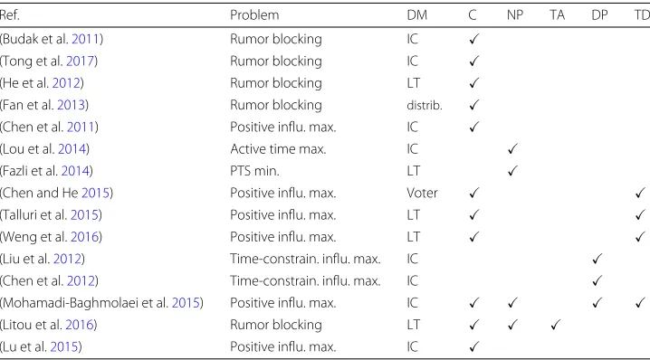
We overview information diffusion models that, in the attempt of explaining realis-tic propagation phenomena, incorporate one or more of the following aspects: multiple, competitive cascades of information, time horizon for the unfolding of the diffusion pro-cess, time-dependent influence, delay in the propagation, trustworthiness of the influence relations. Table1provides a guide to our discussion.
Please note that here we refer to the vast literature on probabilistic models originally designed to explain stochastic processes of information diffusion, which include the clas-sicIndependent Cascade(IC) andLinear Threshold(LT) models (Chen et al.2013), and relating optimization problems, such as influence maximization. By contrast, we will leave out of consideration deterministic models, such as the structural cascades specifically designed to model context/content-sensitive diffusion over an interaction network (e.g., (Krishnan et al.2016; Das et al.2016)). Also, it is worth noting that the information dif-fusion modeling problem we tackle in this work is significantly different from the one addressed byepidemic models, such as SIS, SIR(S), and SEIR(S) (Hethcote2000), already for the non-competitive scenario. Standard epidemic models are originally defined as compartmental models, since the individuals of a population are divided in compart-ments that describe an epidemiological state. The parameters used to represent transition rates for changing states are absolute constants, which means that the infection process in compartmental models has a deterministic behavior. Also, standard epidemic mod-els are of mass-action type, since individuals are represented as normalized fraction of a population which randomly interact with each other. As discussed in (Dodds 2018), even social contagion based on stochastic or generalized epidemic models (i.e., there is
Table 1Summary of related work based on optimization problem, basic diffusion model (DM), competitive diffusion (C), non-progressivity (NP), time-aware activation (TA), delayed propagation (DP), trust/distrust relations (TD)
Ref. Problem DM C NP TA DP TD
(Budak et al.2011) Rumor blocking IC
(Tong et al.2017) Rumor blocking IC
(He et al.2012) Rumor blocking LT
(Fan et al.2013) Rumor blocking distrib.
(Chen et al.2011) Positive influ. max. IC
(Lou et al.2014) Active time max. IC
(Fazli et al.2014) PTS min. LT
(Chen and He2015) Positive influ. max. Voter
(Talluri et al.2015) Positive influ. max. LT
(Weng et al.2016) Positive influ. max. LT
(Liu et al.2012) Time-constrain. influ. max. IC
(Chen et al.2012) Time-constrain. influ. max. IC
(Mohamadi-Baghmolaei et al.2015) Positive influ. max. IC
(Litou et al.2016) Rumor blocking LT
a probability distribution of rates to govern the infection process) is originally defined on random networks, and its revision to deal with social networks would lead to more complicated models. In this regard, one direction is taken by thestochastic individual-contact, network models, whereby SIS and related models are reformulated by considering a stochastic infection process and a network-based population of individually identifiable elements. In “Comparison with the IC, SIR and SEIR models” section, we present a stage of experimental evaluation devoted to a comparison with such models. However, even if epidemic models have also been used for social influence, they are not the most common approach to such topic (Porter and Gleeson2016). This is manly due to the fact that iden-tifying and modeling the causal mechanisms of the spread of ideas is more difficult than for the spread of diseases. By constrast, the threshold models for influence propagation (even the simplest ones) have two important features that are not clearly present in epi-demic models. First, individuals have different behaviors, being such differences reflected in the distribution of activation thresholds associated with the individuals; by contrast, in stochastic epidemic models, the state-transition probabilities are drawn independently of the individuals’ relations. Second, an individual’s behavior also depends on the behavior of other individuals s/he is linked to: here, it is helpful to think about threshold models as an example of complex contagions, whereby an individual takes an action as a result of the exposure to multiple sources of influence; by contrast, epidemic models are more likely to represent simple contagion, in that a single source of influence (as social contact) may suffice to cause an individual’s action. Moreover, while the transition to the recovered state assumes non-progressivity in stochastic diffusion models such as LT or IC, such a transition in SIR(S) is defined to happen spontaneously, discarding any influence that may result from the interaction with other individuals. For all such reasons, thresholds models are usually considered more appropriate in contexts like the adoption of new technolo-gies or controversial ideas (Chen et al.2013). And, in our work, we indeed follow this line of research. One further point of divergence adheres to the notion of competitiveness that is somehow found in advanced epidemic models: this refers to the presence of two or multiple groups of individuals (with some distinguishing characteristics) which are how-ever affected by the same, single disease (Han et al.2003; Ji et al.2012; Hu et al.2013), therefore it corresponds to a totally different notion than what is addressed in our work.
In the following, we briefly recall the definition of the LT model, which is at the basis of our proposal; then, we focus on related work that address the aforementioned aspects concerning complex propagation phenomena.
The classic Linear Threshold model.Given a directed graph representing a social network, with estimates of influence probabilities provided as edge weights, nodes can be “activated” (i.e., influenced) through an information cascade starting from an initially selected set of seed nodes (i.e., early-adopters). At the beginning of the information dif-fusion process, each node is assigned a threshold uniformly at random from [0, 1]. The diffusion process unfolds in discrete time steps and follows certain rules: nodes are either active or inactive; once activated, nodes cannot deactivate; an active node may trigger activation of neighboring nodes; a node can be activated at timet+1 by its active neigh-bors if their total influence weight at timetexceeds the threshold associated to that node. The process runs until no more activations are possible.
competitive diffusion models. Focusing on competitive diffusion and related optimiza-tion problems under the context of misinformaoptimiza-tion spread limitaoptimiza-tion, one of the earliest work is (Budak et al.2011), which proposes a multi-campaign IC model to address the influence limitation problem, i.e., to find a seed set of sizekfor one, “good” campaign such that the number of nodes influenced by the other, “bad” campaign is minimized. In (Tong et al.2017), the problem of rumor blocking is addressed under the competitive IC model and a randomized algorithm is developed for the selection of the seed set able to yield the maximum reduction in the number of bad-infected nodes. An influence block-ing maximization problem is also addressed in (He et al.2012), using competitive LT. In (Chen et al.2011), the two competing cascades correspond to opposite opinions, where the negative one may emerge spontaneously from any user in the network, e.g., a user got disappointed with a purchased item and decides to spread negative opinion among her/his contacts. Lu et al. (2015) also address the aspect of complementarity between two competing campaigns, under the assumption that if the two information items are corre-lated then the adoption of one item might favor further adoption of the second item over time.
Non-progressive diffusion. While modeling the competitive nature of information cascades, the above works however refer to progressive models. On the contrary, a few studies have been proposed to model non-progressive diffusion. For instance, (Lou et al.2014) introduces a deactivation function into a continuous non-progressive model, whereas an extension of LT is proposed in (Fazli et al.2014) to define a non-progressive strict majority model. However, both models are also non-competitive.
Social ties and temporal aspects.All of the aforementioned works discard two impor-tant aspects: (i) the nature of social ties and their impact on the influence propagation, and (ii) time aspects concerning the diffusion process. The dichotomy between opposite types of social ties (e.g., friend vs. foe relations) has been widely studied in OSN analysis (e.g., (Leskovec et al.2010b)), however its incorporation into diffusion models has been rela-tively little explored so far. For instance, two extensions of competitive LT with negative relations are defined in Talluri et al. (2015), to support positive opinion maximization, and in Weng et al. (2016), to model the adoption of opinions from friends or opposite opin-ions from foes. All of such models are competitive but do not consider temporal aspects in the activation or propagation processes.
Dynamic behaviors.All of the previously mentioned works still lack aspects model-ing the dynamic behavior of the users. In particular, accordmodel-ing to recent studies about polarization of opinion in OSNs (Anagnostopoulos et al.2015) and related works about misinformation reduction (Kumar and Geethakumari2014; Lewandowsky et al.2012), a crucial aspect is to intervene before a competing campaign can reach the users, or at least soon enough, so that a user does not have time to radicalize her/his thoughts. This idea was first captured in (Litou et al.2016), where a dynamic LT model (DLT) is defined to deal with competitive information cascades. The influence weights temporally decay according to a Poisson distribution, and every node can be either positively or negatively activated at a given time depending on the absolute value of the cumulative influence of its neighbors, while the activation sign depends on the sign of the cumulative influ-ence. Moreover, a dynamic behavior aspect lays on the update of the activation threshold whenever a user switches her/his belief.
The latter work shares with our proposal all features of competitiveness, non-progressivity (although deactivation is not allowed), time-aware propagation, dynamic influence behavior, and incorporation of opposite opinions in the influence probabilities; moreover, it is also based on LT. However, our competitive models differ from DLT in (Litou et al.2016) since (i) we explicitly model trust and distrust relationships to define the influence probabilities, (ii) our activation function takes into account only the trusted connections while (iii) distinguishing between the two information cascades; (iv) we introduce a quiescence function to model a delay in the information propagation depend-ing on the strength of influence exerted by distrust relations (i.e., foe neighbors); finally, (v) the activation threshold in our models becomes stronger over time as a node is hold-ing a particular belief. In “Comparison with the DLT model” section we shall compare our models with DLT.
Friend-foe dynamic linear threshold models
In this section we describe our proposed class of Friend-Foe Dynamic Linear Thresh-old (F2DLT) models, which is comprised of: the Non-CompetitiveF2DLT(nC-F2DLT), the Semi-Progressive CompetitiveF2DLT(spC-F2DLT), and the Non-Progressive Com-petitiveF2DLT (npC-F2DLT). We first provide an overview of the framework based on F2DLT. Next, we introduce key features common to all models, then we elaborate on each of them.
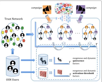
Overview
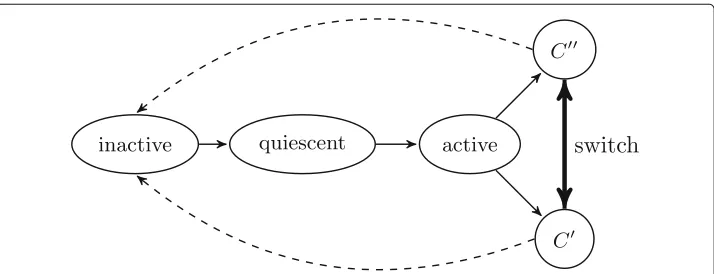
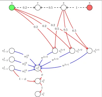
Fig. 1Illustration of the information diffusion framework based on our proposedF2DLT
the information diffusion graph: this also depends on the dynamics of the users’ behav-iors in response to the influence chains started by the campaign(s), which admit that users may switch from the adoption of a campaign’s item to that of another one. Putting it all together, our F2DLT based framework embeds all previously discussed aspects that are required to explain complex propagation phenomena, i.e., competitive diffu-sion, non-progressivity, time-aware activation, delayed propagation, and trust/distrust relations.
Basic definitions
We are given atrust networkrepresented by a directed graphG= V,E,w, with set of nodesV, set of edgesE, and weighting functionw:E→[−1, 1] such that, for every edge (u,v) ∈ E,wuv := w(u,v)expresses how muchvtrusts its in-neighboru. Positive, resp.
negative, value ofwuvcorresponds to atrust, resp.distrust, relation.
For everyv ∈ V, we denote with N+in(v)andN−in(v) the set of neighbors trusted by v(i.e.,friendsofv) and the set of neighbors distrusted byv(i.e.,foesofv), respectively. Moreover, as required in linear threshold models, the constraintsu∈Nin
+(v)wuv≤1 and
u∈Nin
−(v)|wuv| ≤1 must be fulfilled.
LetG = G(g,q,T) = V,E,w,g,q,Tbe a directed weighted graph representing the LT-basedinformation diffusiongraph associated with trust networkG, whereTdenotes a time interval for the diffusion process, g and q denote time-dependent activation-thresholdandquiescencefunctions. These are introduced inG to model the aspects of time-aware activationanddelayed propagation, respectively. We use symbolStto denote
theset of active nodesat timet, and symbolStto denote the set of active nodes for which,
att, the quiescence time is not expired yet, i.e., thequiescent nodes.
Activation-threshold function.According to the LT model, every nodev∈Vis asso-ciated with an exogenous activation-threshold, θv ∈ (0, 1], which corresponds to the a-priori effort needed in terms of cumulative influence to activate the node. We enhance this concept by defining anactivation-thresholdfunction,g : V,T →R+, such that for everyv∈V andt∈T:
g(v,t)=θv+ϑ(θv,t),
i.e., the activation ofvat timetdepends both on the user’s pre-assigned threshold,θv, and
on a time-evolving activation term,ϑ (·,·), which models the dynamic response of a user towards the activation attempt exerted by her/his neighbors.
To specifyϑ (·,·), we devise two main scenarios forg(·,·):
• Abiased scenario, modeled as a non-decreasing monotone function, to capture the tendency of a user to consolidate her/his belief, according to theconfirmation-bias principle (Anagnostopoulos et al.2015).
• Anunbiased scenario, modeled as non-monotone function, whereby we assume that a user could revise her/his uncertainty to activate over time, thus becoming more or less inclined to change her/his opinion on an information item. This is particularly meaningful in applications such as customer retention, or churn prediction (i.e., a decrease in the activation-threshold would correspond to the tendency of a user to churn in favor of another service).
Both variantsϑ (·,·)range within the interval [ 0, 1], for anyv∈V.
Let us first consider the biased scenario, which is focused on the confirmation bias principle. We choose the following form for the activation-threshold function, by which the value increases by increasing the time a node keeps staying in the same active state:
g(v,t)=θv+ϑ(θv,t)=θv+δ×min
1−θv δ ,t−t
last v
, (1)
wheretlast
v denotes the last (i.e., most recent) timevwas activated andδ≥01represents
value, and as a consequence, it will be harder to make the node change its state, or even no more possible (i.e.,g(v,t)saturates to 1, as the differencet−tvlastexceeds(1−θv)/δ).
In the unbiased scenario, we define the activation-threshold function such that, for each v, the value of the function is maximum (i.e., 1) just after the activation, i.e., at timet = tlastv +1, then for subsequent time steps, the function exponentially decreases towardsθv:
g(v,t)=θv+ϑ(θv,t)=θv+exp
−δ
t−tlastv −1
−θvI
t−tlastv =1
, (2)
whereI[·] denotes the indicator function, i.e., it equals 1 ift−tlastv =1, 0 otherwise. Note thatδis used differently w.r.t. the previous scenario, as it acts as a coefficient that controls the decrease of the activation-threshold function over time.
Quiescence function.Each node inGis also associated with aquiescencevalue, which quantifies the latency in propagation through that node. We define aquiescencefunction, q : V,T →T, non-decreasing and monotone, such that for everyv ∈V,t ∈ T, withv activated at timet:
q(v,t)=τv+ψN−in(v),t,
whereτv ∈Trepresents an exogenous term modeling the user’s hesitation in being fully
committed with the propagation process, andψ (N−in(v),t)provides an additional delay proportional to the amount ofv’s neighbors that are distrusted and active, by the time the activation attempt is performed by thev’s trusted neighbors:
q(v,t)=τv+ψN−in(v),t=τv+exp
⎛
⎝λ×
u∈St−1
|wuv|
⎞
⎠, (3)
whereλ≥0 is a coefficient modeling the average user sensitivity in the perceived negative influence. Intuitively, this coefficient would weight more the negative influence as the diffusing informative item is more “worth of suspicion”. Note also that, in Eq.3,wuvis a
negative value, sinceuis a distrusted neighbor ofv, i.e.,u∈N−in(v).
fields (see, e.g., (Tedjamulia et al.2005; Bishop2007)), we believe that the individual’s influenceability has a component based on personal characteristics.
Non-competitive model
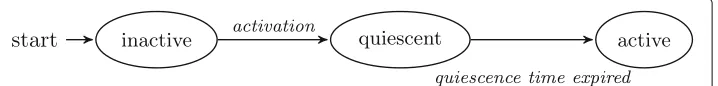
We introduce the first of the three proposed models, which refers to a single-item prop-agation scenario. Figure2shows the life-cycle of a node in the diffusion graph under this model.
Definition 1Non-Competitive Friend-Foe Dynamic Linear Threshold Model (nC-F2DLT)LetG = V,E,w,g,q,Tbe the diffusion graph of Non- Competitive Friend-Foe Dynamic Linear Threshold Model (nC-F2DLT). The diffusion process under the nC-F2DLT model unfolds in discrete time steps. At time t =0, an initial set of nodes S0is activated. At time t ≥ 1, the following rule applies: for any inactive node v ∈ V \St−1∪St−1, ifu∈Nin
+(v)∩St−1wuv ≥ g(v,t), then v will be added to the set of quiescent nodesSt, with quiescence time equal to t∗=q(v,t). Once the quiescence time is expired, v will be removed fromStand added to the set of active nodes St∗. The process continues until T is expired or
no more activation attempts can be performed.
Competitive models
Here we introduce the two competitiveF2DLTmodels. Let us first provide our motivation for developing two different competitive models: through the following example, we illustrate a particular situation that may occur when dealing with two campaigns compet-itively propagating through a network. Please note that, throughout the rest of this paper, we will consider only two competing campaigns for the sake of simplicity; nevertheless, our proposed models are generalizable to more than two competing campaigns.
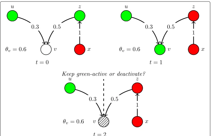
Example 1Figure3 shows an example activation sequence in a competitive scenario between two information cascades, distinguished by colors red and green. At time t = 0, nodes u and z are green-active, and their joint influence causes green-activation of node v as well (since0.3+0.5 ≥0.6). At time t = 1, as fully influenced by node x, node z has switched its activation in favor of the red campaign. After this switch, at time t=2, it hap-pens that v’s activation state is no more consistent with the (joint or individual) influenced exerted by u and z. In particular, two mutually exclusive events might in principle happen at t=2: either v is deactivated or v maintains its green-activation state.
The uncertainty situation depicted in the above example prompted us to the definition of two models, namelysemi-progressiveandnon-progressive F2DLT: the former corre-sponds to the case ofvkeeping its current (i.e., green) activation state, whereas the latter corresponds tovreturning to the inactive state. Clearly, the two models’ semantics are different from each other: the semi-progressive model assumes that a user, once activated,
Fig. 3Uncertainty in an example two-campaign activation sequence
cannot step aside, unlike the non-progressive one, which instead requires a user to have always the support of her/his in-neighbors to keep activation.
Given two information cascades, orcampaigns C,C, for every time stept ∈ T we will use symbolsStandSt to denote the sets of active nodes, such thatSt∩St = ∅, and analogously symbolsStandStas the sets of quiescent nodes, forCandC, respectively. Also,St=St∪St andSt=St∪St.
It should also be noted that, while sharing the time interval (T) of diffusion,CandC are not constrained to start at the same timet0. Nevertheless, for the sake of simplicity, we hereinafter assume thatt0 = t0 = t0 (witht0 ∈ T), unless otherwise specified (cf. “Results” section).
Definition 2Semi-Progressive Competitive Friend-Foe Dynamic Linear Threshold
Model (spC-F2DLT).LetG = V,E,w,g,q,Tbe the diffusion graph of Semi-Progressive
Competitive Friend-Foe Dynamic Linear Threshold Model (spC-F2DLT), and C,Cbe two campaigns onG. The diffusion process under the spC-F2DLT model unfolds in discrete time steps. At time t=0, two initial sets of nodes, S0and S0, are activated for each campaign. At every time step t≥1, the following state-transition rules apply:
R1.For any inactive node v ∈ V \St−1∪St−1
, ifNin
+(v)∩St−1wuv ≥ g(v,t), then v will be added toSt; analogously, ifNin
+(v)∩St−1wuv ≥g(v,t), then v will be added toSt. If both conditions hold, i.e., v can be simultaneously activated by both campaigns, a tie-breaking rule will apply, in order to decide which campaign actually determines the node’s transition in the quiescent state.
R2.When a node v enters the quiescent state corresponding to C(resp. C) for the first time, it will stay in the quiescent node-setSt(resp.St) until the quiescence time is expired.
R3. Given a node v active for C, i.e., v ∈ St−1, ifNin
+(v)∩St−1wuv ≥ g(v,t) and
N+in(v)∩St−1wuv >
N+in(v)∩St−1wuv, then v will be removed from St and added to St;
analogous rule holds for any node active for the first campaign.
Every node for which none of the above transition-state rules is triggered at time t, it will keep its current state at time t+1.
The life-cycle of a node in spC-F2DLT is shown in Fig. 4. Note that, once a node becomes active, it cannot turn back to the inactive state, but it can only change the activation campaign. Moreover, switch transitions occur instantly.
Definition 3Non-Progressive Competitive Friend-Foe Dynamic Linear Threshold
Model (npC-F2DLT)LetG = V,E,w,g,q,Tbe the diffusion graph of Non-Progressive
Competitive Friend-Foe Dynamic Linear Threshold Model (npC-F2DLT), and C,C be two campaigns onG. The diffusion process in npC-F2DLT evolves according to the same rules as in spC-F2DLT plus the following rule concerning the deactivation process of an active node:
R4.For any active node v at time t−1, ifNin
+(v)∩St−1wuv < θvand
N+in(v)∩St−1wuv< θv, then v will turn back to the inactive state at time t.
Every node for which none of the transition-state rules is triggered at time t (including the ones defined for spC-F2DLT), it will keep its current state at time t+1.
It should be noted that a node’s deactivation rule depends onθvonly (rather than on the whole functiong(v,t)); otherwise, every node activated at a given time could deac-tivate itself in the next time step, due to the increase in its activation threshold. This would eventually lead to a configuration in which all nodes in the network, except the ini-tially activated ones, are in the inactive state. The life-cycle of a node in thenpC-F2DLT is illustrated in Fig.4. Note that, unlike inspC-F2DLT, transitions to inactive state are allowed.
Theoretical properties of the models
In this section we provide insights into the proposed models. Our main goal is to under-stand how the features introduced in each of our LT-based models impact on the models’
spread behavior, particularly on monotonicity and submodularity properties. We orga-nize our analysis into two parts: the first corresponding tonon-competitivediffusion, and the second tocompetitivediffusion.
Non-competitive diffusion
We show thatnC-F2DLTcan be reduced toLT with quiescence time, hereinafter denoted asLTqt. By proving the equivalence between the two models, we hence claim that both the monotonicity and submodularity properties hold fornC-F2DLT. Note that since we deal with a progressive model, we assume without loss of generality that, for every nodev, the activation-threshold function has a constant value for the whole duration of the diffusion process, i.e.,g(v,t)=θv.
Definition 4Reduction of nC-F2DLT to LTqt. Given G = V,E,w,g,q,T for nC-F2DLT, a diffusion graphGLT = VLT,ELT can be derived, under LTqt, such that
VLT = V and ELT = {(u,v)|(u,v) ∈ E,wuv > 0}. Every node v ∈ VLT is assigned
a quiescence time equal to the maximum value of the quiescence function qv(·), i.e., τvmax=τv+ψ (N−in(v)).
Definition4exploits the fact that the distrust connections are not involved in the activa-tion process, but only in the calculaactiva-tion of the quiescence time. Therefore, we can assume this time to be the maximum possible value, and hence we can study the propagation underLTqt. The reduction ofnC-F2DLTtoLTqtis meaningful since the two models are proved to be equivalent, as we report in the following theoretical result.
Proposition 1 The Non-Competitive Trust Threshold Model (nC-F2DLT) and the Linear Threshold Model with quiescence time (LTqt) are equivalent.
ProofAccording to the definition of equivalence of two diffusion models in (Kempe et al.2003; Chen et al.2013), in order to prove the equivalence ofnC-F2DLTand LTqtwe need to prove that the distribution of theactive setsfor any given seed setS0is the same under the two models. We provide a proof by induction, hence we consider the evolution of the active sets during the diffusion rounds.
For theLTqtmodel, the probability of a node to be activated exactly at timet+1 (with t≥1) is given by:
Pr(v∈St+1|v∈/St)=
Prv∈St+1,v∈/St
Pr(v∈/St)
= Pr
u∈St−1wuv< θv≤
u∈Stwuv
Pru∈St−1wuv< θv
=
u∈St\St−1wuv 1−u∈St−1wuv
(4)
Above, it should be noted that the joint probability Prv∈St+1,v∈/St
corresponds to the probability that the threshold associated with nodevfalls into the interval denoted by the influence received byvuntil the previous time step and the one received at the current time step. Moreover, Pr(v ∈/ St) is just the probability that, at time(t−1), the
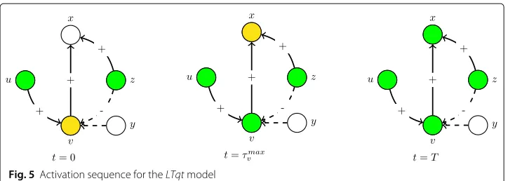
Fig. 5Activation sequence for theLTqtmodel
Eq.4, which intuitively denotes that the influence exerted by the nodes inSt\St−1, i.e., the nodes turning into the active state exactly in the current time step, is decisive to exceed the thresholdθv.
For the npC-F2DLT model, the conditional probability Prv∈St−1|v∈/St
can be derived starting from Eq.4by constrainingwuv such thatu ∈ N+in(v), i.e., only trusted
relations are considered. This leads to an equivalent definition of conditional probability, which holds for every time steptand seed setS0. Therefore, we can conclude that the final active sets will be the same for both models.
It should be noted that, due to the quiescence times, the sets of active nodes in the two models may not be the same at every time step, but the two final active sets will match each other.
Since the introduction of quiescence time in LT does not have effect on the distribution of the final active nodes (Chen et al.2013), we obtain the following equivalence:LT ≡ LTqt≡ nC-F2DLT. Therefore, the activation function is still monotone and submodular undernC-F2DLT.
Example 2Consider Fig.5, where the propagation process unfolds according to the LTqt dynamics. Nodes u and z are chosen as initial seeds. Thresholds and weights are set such thatθ ≤wuvandmax{wvx,wzx} < θx ≤wvx+wzx, therefore the combined influence of v
and z is required for the activation of node x. The dashed edge denotes a distrust connection removed as a result of the reduction defined in Definition4. In the initial time step (t=0), u activates v causing its transition from the inactive state to the quiescent state (in yellow). When t = τvmax, v turns to the active state, and together with z it becomes able to trigger the activation of node x (which will eventually become active by the time-horizon T).
It should be noted that the same dynamics holds for the nC-F2DLT model, apart from the difference that concerns the quiescence time of node v: this would be less thanτvmaxsince y, a foe of v, is not involved in the propagation process.
Competitive diffusion
To begin with, we might recall that the non-progressive LT-based diffusion can be reduced to the progressive case, using a particular form oflayeredgraph (Kempe et al.
2003). Given a time intervalTand a diffusion graphG= V,Efor non-progressive LT, a new graphGTcan be derived such that every nodev∈Vwill have a replicavtin every
layer at timet∈T, and for every edge(u,v)∈Ethere will be an edge(ut−1,vt)inGT.
Unfortunately, this serialization technique cannot be directly applied to our models, since it is not designed to deal with competitive or non-progressive diffusion and it dis-cards activation or delayed propagation aspects. In the following, we define serialization techniques that are suitable for our competitive models and treat one particular con-figuration at a time. One general requirement is related to the time horizon to bound the unfolding of the diffusion process. In fact, when dealing with competitive models, the termination guarantee is lost. A simple example is provided next to depict such a non-termination scenario.
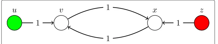
Example 3In Fig. 6, nodes u and z are chosen as seed for the green campaign and the red one, respectively. Nodes v and x become green-active and red-active, respectively, at time t = 1. Next, they will constantly switch their activation campaign, causing
non-termination of the diffusion process.
CONFIGURATION1: No quiescence time, constant activation-threshold. We assume thatq(v)=0 andg(v,t)=θv, for allv∈V,t∈T. For bothspC-F2DLTandnpC-F2DLT, we claim their reduction to the H-CLT model with majority voting as tie-breaking rule.
Definition 5spC-F2DLT graph serialization for reduction to H-CLT.Given a time interval T, we define a layered graph GT = VT,ETsuch that, for each layer at time
t∈ T, every node v∈V will be represented in VT as a tuplev1t,v2t,v3t. Instances v1t and v2t have activation-threshold equal to 0, while v3t has the same threshold as the original node v ∈ V . The set of edges is defined as ET = u1t,v3t+1|(u,v)∈E,t,t+1∈T∪
v3t,v2t|v∈V,t∈T∪v2t,v1t|v∈V,t∈T∪v1t,v2t+1|v∈V,t∈T, and the following constraint on edge weights must hold:∀v2t ∈VT, wv1t−1,v2t<wv3t,v2t.
In the above definition, triples act asconnectorsbetween two consecutive time-layers. The role of any connector component is as a sort of “switch” to enable a node choosing between its activation state in a layer and the one in the subsequent layer. In other words, nodev1t is the main instance of nodev, since the activation state ofv1t reflects the state of vin the original graph, underspC-F2DLTat timet; nodev3t is the instance ofvconnected with other nodes from layer att−1, therefore it reflects the influence received byvin the
original graph, at timet−1; if the activation attempt tov3t fails, nodev2t will be activated with the same state ofv; otherwise, according to the edge weight constraint (cf. Defini-tion5),v2twill switch to the other campaign, and then will propagate to instancev1t. Recall thatv1t,v2t have zero activation-threshold. Figure 18 in AppendixAshows an example of serialization for aspC-F2DLTdiffusion graph with time horizon set to 2.
It should be emphasized that, compared to the serialization method in (Kempe et al.
2003), we require replication of each node in each layer, and additional edges connecting the replica-instances, in order to allow the maintenance of the activation state when no activation event occurs between two time-consecutive layers.
Analogous reduction technique can be defined for thenpC-F2DLTmodel.
Definition 6npC-F2DLT graph serialization for reduction to H-CLT.Given a time interval T, we define a layered graph GT = VT,ETsuch that, for each layer at time t ∈ T, every node v ∈ V will be represented in VT as a tuple vt1,v2t,v3t. Instances v1t and v2t have activation-threshold equal to 1 and 0, respectively, while v3t has the same threshold as the original node v ∈ V . The set of edges is defined as ET =
u1t,v3t+1|(u,v)∈E,t,t+1∈T∪v3t,vt2|v∈V,t∈T∪vt2,v1t|v∈V,t∈T∪
v3t,v1t|v∈V,t∈T∪vt1,v2t+1|v∈V,t,t+1∈T, and the following constraints on edge weights must hold:∀v2t ∈VT, wv1t−1,v2t<wvt3,v2t, and∀v1t ∈VT, wv2t,v1t+ wv3t,v1t=1.
It should be noted that the last condition in Definition6imposes nodesv2t andv3t to hold the same activation state in order to activatev3t.
Analogously to the reduction ofspC-F2DLT toH-CLT, we can conveniently devise a notion of “connector” component between any two consecutive layers, which however in this case should also account for node deactivations. Figure 19 in AppendixAshows an example of connector for thenpC-F2DLTmodel.
Claim 1For any given diffusion graphGunder spC-F2DLT (resp. npC-F2DLT), assum-ing constant activation-threshold and no quiescence time, every node v inG is active at time t∈T if and only if its corresponding instance v1t is active in the serialized graph GT
(resp. npC-F2DLT).
CONFIGURATION2: Constant quiescence time, constant activation-threshold. We assume that q(v) = τv and g(v,t) = θv, for all v ∈ V. For both spC-F2DLT and npC-F2DLT, we claim their reduction toH-CLTwith majority voting as tie-breaking rule. In this case, we need to consider that, whenever a node is activated, its quiescence time may not expire before the time horizon; for this reason, we will consider only nodes reachable fromS0 = S0 ∪S0 withinT, for any two given seed setsS0andS0. To iden-tify such nodes, we define aquiescence-aware distance measure that accounts for the quiescence times along the path connecting any two nodes. Given nodesu,v, and the set P(u,v) of all paths betweenuandv, the distance fromu tovwill be measured as d(u,v) =minp∈P(u,v)x∈pτx. Moreover, we denote withd(S0,v)the minimum distance between nodesu ∈ S0andv. By exploiting this distance, we will discard all nodes that cannot be “contagious” before the end ofT, saytmax. Therefore, the node setVT of the
VT =v1t,v2t,v3t| ∀v∈V, t∈T, d(S0,v) <tmax
.
Each nodev ∈ V with quiescence time τv will have connections from the previous layers according to the following rule: for any layer at timet, ift<d(S0,v)thenvwill not have any incoming edges, otherwise all incoming edges ofvwill be from the layer at time t−τv−1.
Using the above settings in the serialization method previously presented, it can easily be demonstrated that bothspC-F2DLTandnpC-F2DLTcan be reduced to an equivalent H-CLTmodel.
Claim 2For any given diffusion graphGunder spC-F2DLT (resp. npC-F2DLT), assum-ing constant activation-threshold and constant quiescence time, every node v inGis active at time t ∈ T if and only if its corresponding instance v1t is active in the serialized graph
GT(resp. npC-F2DLT).
CONFIGURATION 3: Variable quiescence time, constant activation-threshold. We assume thatq(v,t)is variable, whileg(v,t)=θv, for allv∈V,t∈T.
Like in the previous case, we need to specify the seed setsS0,S0. However, note that the quiescence time of a node now depends on the actual activation state of its in-neighborhood (cf. Eq.3), which makes it unfeasible a direct serialization of the whole diffusion graph.
Starting from the original diffusion graphG, we derive an “intermediate” graphG, which is equivalent toGunless each nodev∈ V is associated with a quiescence time interval [τv,τvmax], whereτvmax=τv+ψ (N−in(v)). Let us denote withGminthe instance ofGsuch
that the quiescence time of everyv∈Gisτv, and withGmaxthe instance ofGsuch that
the quiescence time of everyv∈Gisτvmax.
Although we cannot assert that spC-F2DLT and npC-F2DLT are equivalent to H-CLTunder the layered graph obtained by applying the previously described serialization techniques, an important theoretical result can nonetheless be provided, as reported next.
Claim 3For any diffusion graph Gunder spC-F2DLT (resp. npC-F2DLT), with cam-paigns C,C, assuming constant activation-threshold and variable quiescence time, for any seed sets S0and S0, it holds that:
σH−CLTmax (S0,S0)≤σ(S0,S0)≤σH-CLTmin (S0,S0), (5)
whereσ is the number of nodes activated by Cunder spC-F2DLT (resp. npC-F2DLT), σH-CLTmax (S0,S0)andσH-CLTmin (S0,S0)are the number of nodes activated by Cunder H-CLT in the layered graph obtained by serialization of spC-F2DLT (resp. npC-F2DLT) on
GmaxandGmin, respectively.
Enabling variable quiescence time, i.e.,ψ (·), means that the exact time required by each node to make a transition from the quiescent state to the active one cannot be established in advance at the beginning of the propagation process. Since for any nodevthe quies-cent time ranges within [τv,τvmax], we devise two opposite scenarios. In the first scenario,
by the leftmost side of Eq.5, assumes that each node has to wait the maximum possible quiescence time, i.e.,τmax; as a consequence, a smaller fraction of nodes will be able to complete the activation process before the time limit, thus leading to a lower spread.
CONFIGURATION4: No quiescence time, variable activation-threshold. We assume thatq(v) = 0 andg(v,t) = θv+ϑ (θv,t), for allv∈V,t ∈T. For bothspC-F2DLTand
npC-F2DLT, we claim their reduction toH−CLT with majority voting as tie-breaking rule. In the following, we refer to the biased activation-threshold function, although it is easy to show analogous considerations for the non-biased activation-threshold function.
Because of the dynamic behavior of the activation-threshold function, we cannot predict its value at any particular time step of the diffusion process; nevertheless, by spec-ifying the value of coefficientδ in Eq.1, we can derive the value oftmax
v , which would
suggest how many time-layers we have to look back in order to know the actual thresh-old value ofvat a particular timet. In order to capture such dynamic aspect inH-CLT, we define a further serialization technique, built on top of the previously defined. We will restrict to a particular case, afterwards we provide some rules that apply to the general case.
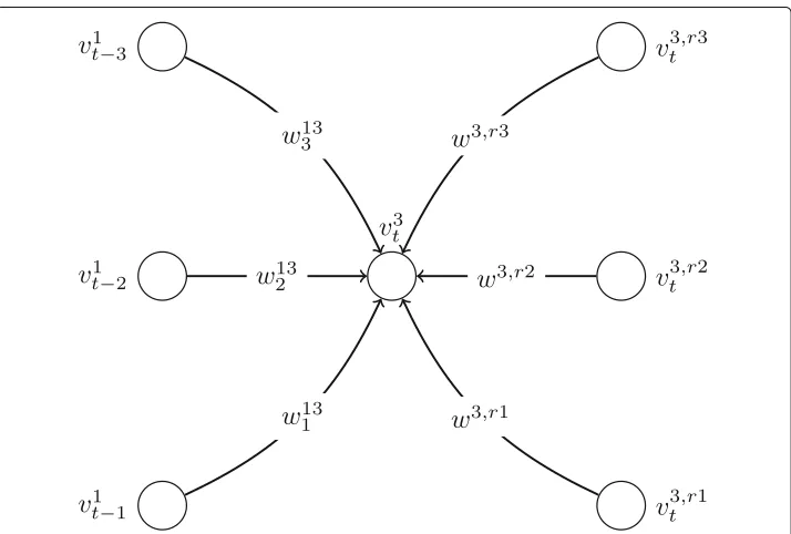
Let us assume to focus on a particular nodev, and at any two consecutive time steps of activation for the same campaign its threshold increases byδ. Again, nodevwill have replicasfor any time-layert, i.e.,v1t,vt2,v3t, with the first replica,v1t, holding the actual state ofvin the corresponding serialized graph for the competitive model. In addition, we introduce further replicas, in number equal to the valuetvmax; suppose, for the sake of simplicity,tmaxv = 3, we derive replica nodesv3,tr1,v3,tr2,v3,tr3, such that each of them will have a threshold value in [θv, 1] with increment ofδ. Figure 7illustrates this new
component in the serialized graph.
Because this component is introduced as an extension of the previous techniques, the meaning of the nodesv1t−1,v1t−2,v1t−3remains the same as in the previous cases. On the right side of Fig.7, each of the additional replicas has a different value of threshold and it is connected with nodes coming from the previous layers. Clearly, the overall behavior of this component depends on the weights attached to every edge in the structure. In this regard, we define the following constraints on the edge weights:
⎧ ⎪ ⎪ ⎪ ⎪ ⎪ ⎪ ⎨ ⎪ ⎪ ⎪ ⎪ ⎪ ⎪ ⎩
w3,r1>w13
1 (a)
∀i>1 w13i =w3,ri (b) ∀i≥1 w13i >nj>iw13j (c) ∀i≥1 w3,ri>nj>iw3,rj (d) w3,r1−w13
1 <w13n (e)
(6)
It should be noted that the activation attempts are performed directly on the replicas. Therefore, the above constraints on the edge weights control whether a node assumes the state derived as the outcome of the most recent activation attempts, or the one consistent with its personal history. as the outcome of the most recent activation attempts or the one consistent with its personal history. Each of the aforementioned inequality contributes to this decision process, following a different purpose. Eq.6(a) ensures that the state derived from the last activation attempt is always preferred to the one derived from the previous time step. Eq.6(b) ensures that the information coming from the previous time steps shall be given the same importance as the one derived from the current replicas. Eq.6(c-d) ensures that the most recent information, i.e., the closest previous time steps, has higher priority than the earliest one. Eq.6(e) ensures that there is consistency with respect to the state assumed in the closest previous time step and farthest involved time step (e.g., the third previous time step in the addressed scenario).
Moreover, the threshold of the “central” node in the component (v3t) is set tow3,r1, to ensure sequentiality of the diffusion. By settingθv3
t equal tow
3,r1, we avoid thatv3
t can be
activated by its own replicas belonging to layers preceding thet−1-th layer.
Figure8shows how the above defined connector is integrated into a serialization tech-nique. In the figure, only the connections incident on vertexvare expanded. The red edges are the ones connecting consecutive layers, therefore the replicav3,tr1is connected with the previous layer, the replicav3,tr2is connected with the second previous layer and so on. Blue edges represent the new connections due to the introduction of this new component.
Claim 4For any given diffusion graphGunder spC-F2DLT (resp. npC-F2DLT), assum-ing variable activation-threshold and no quiescence time, every node v inGis active at time t∈T if and only if its corresponding instance v1t is active in the serialized graph GT
(resp. npC-F2DLT).
Evaluation methodology Data
We used four real-world, publicly available networks, namely:Epinions(Leskovec et al.
Fig. 8Serialization of a diffusion graph under a competitive model with time-varying activation-threshold
in an “edit-war”, i.e., edges represent either positive or negative conflicts in editing a wikipage. Wiki-Vote models “who-vote-whom” relations between Wikipedia users that voted for/against each other in admin elections. Our choice of the evaluation datasets was mainly driven by two intents: (i) to provide a reproducible evaluation framework based on publicly available network data, and (ii) to test our models on a diversified set of real-world OSNs with suitable characteristics for information propagation processes.
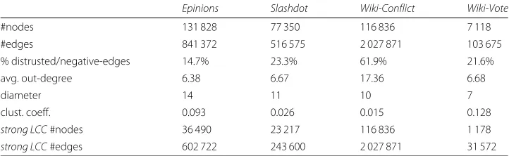
Table2 summarizes main structural characteristics of the networks. To favor mean-ingful competition of campaigns based on selected pairs of strategies, we limited the diffusion context to the largest strongly connected component in each evaluation net-work; note that, for Wiki-Conflict, the largest strongly connected component coincides with the whole graph. Also, the clustering coefficient corresponds to the definition of global transitivity in an undirected graph (the direction of the edges is ignored).
All networks are originally directed and signed; in addition, the two Wikipedia-based networks also have timestamped edges. In order to derive the weighted graphs of influ-ence probabilities, we defined the following method: for every(u,v)∈E, the edge weight wuvwas sampled from a binomial distributionB
|N+in(v)|,pifu ∈ N+in(v)(i.e.,vtrusts u), otherwisewuv ∼ −B
Table 2Summary of evaluation network data
Epinions Slashdot Wiki-Conflict Wiki-Vote
#nodes 131 828 77 350 116 836 7 118
#edges 841 372 516 575 2 027 871 103 675
% distrusted/negative-edges 14.7% 23.3% 61.9% 21.6%
avg. out-degree 6.38 6.67 17.36 6.68
diameter 14 11 10 7
clust. coeff. 0.093 0.026 0.015 0.128
strong LCC#nodes 36 490 23 217 116 836 1 178
strong LCC#edges 602 722 243 600 2 027 871 31 572
each node is more likely to be involved in the propagation process. We performed 1000 samplings of edge weights, for each of the four networks. Therefore, all presented results will correspond toaverages of 1000 simulation runs.
Seed selection strategies
We defined four seed selection strategies, each of which mimics a different, realistic scenario of influence propagation.
Exogenous and malicious sources of information.This method, hereinafter referred to asM-Sources, aims at simulating the presence of multiple sources of malicious informa-tion within the network. Here, an exogenous source is meant as a node without incoming links, e.g., a user that is just interested in spreading her/his opinion: such a node is also regarded as malicious if a high fraction of outgoing influence exerted by the node is dis-trusted by out-neighbors. Formally, given a budgetk, the method selects the top-kusers in a ranking solution determined asr(v) = (W¯−/(W¯−+ ¯W+))log(|Nout(v)|), for every vsuch thatNin(v)= ∅, whereW¯ +,W¯−are shortcut symbols to denote the sum of trust (resp. distrust) weights, respectively, outgoing fromv.
Exogenous and influential trusted sources of information.Analogously to the previ-ous method, this one, dubbedI-Sources, searches for the “best” influential trusted sources. The ranking function is asr(v) = (W¯+/(W¯−+ ¯W+))log(|Nout(v)|). Note that this still takes into account the negative weights, because even a highly trusted user might be distrusted by some other users (e.g., “haters”).
Stress triads. This strategy is based on the notion of structural balance in triads (Leskovec et al.2010b). Figure9shows an example of stress-triad configuration: nodev has two incoming connections, the one from nodezwith negative weight, and the other fromuwith positive weight, and there is also a trust link fromztou. We say thatzis astress-nodesince, despite the distrusted link tov, it could also indirectly influencev through the trusted connection withu. Based on that, our proposedStress-Triadsstrategy searches for all triads containing stress-nodes and selects as seeds the firstkstress-nodes with the highest number of triads they participate to.
Fig. 9Stress configuration
those with the oldest start-time and with the newest start-time, respectively. Both strate-gies were applied to Wiki-Vote and Wiki-Conflict, due to the availability of timestamped edges.
Settings of the model parameters
For every userv, the exogenous activation-thresholdθvand quiescence timeτvwere
cho-sen uniformly at random within [0,1] and [0,5]. Moreover, λ (used in the quiescence function) was varied between 0 and 5, while the coefficient δ (used in the activation-threshold function) was selected in{0, 0.1}for the biased scenario (Eq.1) and kept fixed to 1 for the unbiased scenario (Eq.2).
Results
We organize the presentation of our experimental results into three parts. The first part is devoted to the evaluation of the non-competitive model (“Evaluation ofnC-F2DLT”
section), and the second part for the competitive models (“Evaluation of competitive models” section). In the third part (“Comparative evaluation” section), we present a comparative evaluation of our non-competitive model against IC and stochastic individual-contact epidemic models, whereas for the competitive scenario, we compare our models with the DLT model (Litou et al.2016).
Evaluation ofnC-F2DLT
Spread, stressed users and negative influence
a
b
c
d
Fig. 10 Spread ofnC-F2DLTby varying seed set size (k) and selection strategy.aEpinions, I-Sources.b
Slashdot, M-Sources.cWiki-Vote, Stress-Triads.dWiki-Conflict, Most-New
withLeast-Newprevailing onMost-Newfor lowerk. By contrast,M-Sourceswas in general unable to yield a spread comparable to other strategies.
Table 3Summary about negative influence spread (k=50) Strategy
M-Sources I-Sources Stress-Triads Most-New Least-New Network
Epinions # nodes 0 2 117 847 -
-avg weight 0 0.30 0.22 -
-Slashdot # nodes 0 4 599 345 -
-avg weight 0 0.32 0.19 -
-Wiki-Conflict # nodes 13 829 26 1 0
avg weight 0.22 0.05 0.01 0.02 0
Wiki-Vote # nodes 45 27 175 10 12
avg weight 0.21 0.13 0.22 0.04 0.07
Activation loss
As partially unveiled by the previous analysis, the users’ involvement in the propaga-tion process is affected by the behavior of the quiescence funcpropaga-tion, whose impact would increase with the amount of distrusted influence in the spread. This further prompted us to measure theactivation loss, i.e., the percentage decrease of activated users, due to the enabling of the time-varying quiescence factor (i.e.,λ > 0 in Eq.3) in the users’ activa-tion states. Figure11shows results corresponding to relatively largeλ(set to 5) andk(set to 50). For each seed selection strategy, the curve is drawn by using polynomial splines,2 where the marked points (from low to high time steps) refer to the 25%, 50%, 75% and 100% of the time horizon observed for the diffusion process under the chosen strategy without time-varying quiescence times. One general remark that stands out is a relatively high percentage of activation loss for the initial time steps; this holds in particular for Stress-Triads, which might be explained since the initial influenced users by means of this strategy tend to be subjected to a certain amount of distrusted influence. As the time steps get closer to the time horizon, the activation loss tends to significantly decrease, down to nearly zero in most cases, with few exceptions including the use ofI-Sourcesin Slash-dot and Epinions, andStress-TriadsandM-Sourcesin Wiki-Vote — note this is indeed consistent with the previous analysis on negative influence spread.
Evaluation of competitive models
To analyze the behavior ofspC-F2DLT andnpC-F2DLT, we aimed at simulating a sce-nario oflimitation of misinformation spread, i.e., we assumed that one campaign, the “bad” one, has started diffusing, and consequently another campaign, the “good” one, is carried out in reaction to the first campaign.
Combining seed selection strategies
a
b
c
d
Fig. 11 Activation loss due to time-varying quiescence (forλ=5,k=50) under thenC-F2DLTmodel.a Epinions.bSlashdot.cWiki-Conflict.dWiki-Vote
Setting and goals for the evaluation of competitive diffusion
As previously mentioned, the seed selection strategies chosen for the two campaigns might not start at the same time, in which case we assume that the first-started one is the bad campaign. Moreover, we used fixed-probability as tie-breaking rule, with probabil-ity equal to 1 for the bad campaign. Also, we set the time horizon to the end-time of the (non-competitive) diffusion of the bad campaign.
Our main goal in the analysis of the two competitive models was to understand the effect of the setting of the activation-threshold function on the users’ campaign-changes/deactivations, under the case of “real-time correction” or “delayed correction” by the good campaign against the bad one (cf. Introduction).
Evaluation of spC-F2DLT
a b c
d e f
Fig. 12 spC-F2DLT: Spread, number of switched users, and number of switches (log scale) by varying start-delay (t0) of the “good” campaign (second bars), forδ=0 (left-most bar groups) andδ=0.1 (right-most bar groups),k=50.aEpinions.bSlashdot.cWiki-Conflict.dWiki-Conflict.eWiki-Vote.fWiki-Vote
to start-delayst0of the good campaign w.r.t. the bad one (from 0 to 75% of the end-time of the bad campaign). For this analysis, we considered the biased definition of the activation-threshold function (Eq.1).
One general remark is that, forδ = 0,t0 = 0, the seed strategy that showed to be most effective in spread in the non-competitive case (cf. Table4) confirmed its advan-tage against the other campaign’s strategy. Nevertheless, forδ > 0,t0 > 0, the two campaigns would tend to an equilibrium, or even to invert their trend (e.g., in Epinions and Wiki-Vote). In particular, by accounting for (even little) confirmation bias and let-ting both campaigns start at the same time,I-Sourcesslightly increases its spread (which is explained since this strategy allows for activating first a high fraction of shared users, e.g., 70% in Epinions); but, as the start-delay increases at 50%, the good campaign is no more able to save users from being influenced by the bad campaign (i.e.,Stress-Triadsin Epinions,M-Sourcesin Wiki-Vote).
Interesting remarks were also drawn from the analysis of the transitions from one campaign to the other one. For δ = 0, as the start-delay increases, the number of switched users follows a nearly constant trend in all networks (but Wiki-Vote, where we observed a drastic decrease for both campaigns), while the total number of switches is subjected to a more evident decreasing trend. Moreover, we observed a higher num-ber of (unique and total) switches from the bad campaign to the good campaign, than vice versa, which occurred even when the spread of the bad campaign was higher than the good one (e.g., in Wiki-Vote, for both combinations of strategy choices). Setting δ = 0.1 led to a general decrease in the switch measurements w.r.t. the correspond-ing previous case, and also to a substantial increase in “saved” users by the good campaign.