Lincoln
University
Digital
Thesis
Copyright
Statement
The
digital
copy
of
this
thesis
is
protected
by
the
Copyright
Act
1994
(New
Zealand).
This
thesis
may
be
consulted
by
you,
provided
you
comply
with
the
provisions
of
the
Act
and
the
following
conditions
of
use:
you
will
use
the
copy
only
for
the
purposes
of
research
or
private
study
you
will
recognise
the
author's
right
to
be
identified
as
the
author
of
the
thesis
and
due
acknowledgement
will
be
made
to
the
author
where
appropriate
you
will
obtain
the
author's
permission
before
publishing
any
material
from
the
thesis.
The structure of global invasive species
assemblages and their relationship to
regional habitat variables: converting
scientically relevant data into decision
relevant information.
A thesis
submitted in partial fullment of the requirements for the Degree of
Doctor of Philosophy at
Lincoln University
by
Mariona Roigé Valiente
Abstract
Quantitative methods for pest risk assessment combine sound statistical tools with sound ecological theory to convert scientically relevant data into decision-relevant information. This thesis investigated a quantitative method for pest risk assessment called pest prole analysis (PPA). PPA is a new methodology that is based on the premise that the risk of invasion by crop pests into new areas can be predicted by analysing regional insect pest assemblages (also known as pest proles). Regional pest assemblages comprise the presence or absence of recognised pest species in each region of the world. The analysis involves clustering these regions based on similarities between their pest proles. PPA assumes that co-occurrence of pest species in a region is the outcome of a non-random structured process driven by biotic and abiotic characteristics of the region. The most commonly used clustering technique for grouping regional pest assemblages is a self-organizing map (SOM), which is an articial neural network algorithm. Two other clustering methods that have also been used for PPA are hierarchical clustering (HC) and k-means. The main aim of this thesis was to perform a thorough validation test of the PPA approach. To do so, I rst analysed the sensitivity of SOM PPA to changes in the number of species used as input data. The results showed that SOM PPA outputs (weight values that are interpreted as risk indices) were quite sensitive to changes in the input data. However, when the risk indices were transformed into ranked lists of species, the ranks were signicantly less sensitive and hence potentially more useful for pest risk assessment. I assessed the validity of the groups (clusters) of regions obtained from a SOM PPA by applying an external validation measure, the ζ diversity metric. The ζ metric was used to quantify similarities between
Acknowledgments
I feel the need to acknowledge and thank everyone along the way. And that is going to be long because I am submitting this thesis after an enjoyable and well-lived education path that lasted 30 years. I had an early start and took it easy. I started school at kindergarten Montisbel when I was still not one year old. Thanks Senyoreta Montse and Senyoreta Tina for teaching me how to read, how to write and how to make those amazing penne pasta necklaces that I wore with so much pride.
Thanks to my primary school, La Salle Palamos, for its big sandy playground, for the amazing stone stairs where we took the end-of-the-school-year pictures and where so many other life-changing things happened for the rst time. And thanks Rodri, for being the 4th grade teacher every 9 years old in the world deserves to have in their life.
Special thanks go to my secondary high school, IES Palamos, where I learned that the world was a much bigger place than what I thought before, where I met Javi, who, by inscrutable means, is still a part of my life today. Thanks Nuria Corredor, before writing in a public forum, I always think about you, and about how embarrassed I would be to disappoint you by misspelling a Catalan word.
Then, University of Girona was the place where I graduated as an Economist and then obtained my masters in Environmental Sciences. Without the thoughtful mentoring and advice from Gemma Renart, Diego Varga, Marc Saez, and Andreas Kyriacou that would never have happened. Seriously, never!
I extend abundant and sincere thanks to the rest of my co-supervision team, Dr. Craig Phillips for being the best language editor that a non-English speaker can ever dream of, among many other qualities. Also thanks so much Dr.Matthew Parry for the patience and your ability to put extremely complex concepts in understandable words that even I could grasp. You have been very useful and I appreciate it so much. I would also like to thank my collaborators in Monash University, Associate Professor Melodie A.McGeoch and Professor Cang Hui from Stellenbosch University for allowing me to work at a top-level project hands on with them.
Thanks to all the Ecological Informatics department, to the ones that stayed and the ones who went on with their amazing careers elsewhere. Dr.Hossein Ali Narouei Khandan, Jack Linton (my favourite summer scholar ever), Marona Rovira Capdevila, Ursula Torres and Dr.Senait Senay. And very special merci beaucoup to my very special Dr. Audrey Lustig, whose last name stands for 'merry' or 'cheerful' in English, and she has taught me more than what she will ever realize.
To the friends I left in the northern hemisphere, most of whom are today spread throughout the world, I miss you, think you and thank you. Nuria Abad, Marjorie Aznar, Deli Moreno (and Fletxa), Dani Sanchez (where are you now?), Marc Melus, Pau Mora, Joan Romans, Estibaliz Herranz (and Trap and Fion), Nahia Canibe, and my two little ones (with their two little ones), Sonia Cabezon and Natalia Abascal, and Nahia and Ona. To the friends I gained in the southern hemisphere. New Zealand without you would just have been a bit less great. Martona (`hemos sabido volver a encontranos'), Gabriel (whatever I write here, it won't be special enough), Ursu (`the best you can is good enough'), SimonLimón , Cucaracha, Laura, Marjon, Damià, Dede, Sam, Andy, Mark, Bruno, Marona, Euge, Fede, Cesco, Aimee, Pri, Majo, Richard, Ruth, Pavi, Mauricio, Fanny, Cian, Nia, Yann and all those that are still to come.
Contents
Abstract . . . i
Acknowledgments . . . iii
List of Figures . . . xi
List of Tables . . . xiii
1 General introduction . . . 1
1.1 Biological invasions and Biosecurity . . . 1
1.1.1 Biosecurity: Policies, Agencies and Pest Risk Analysis . . . 4
1.1.1.1 Pest Risk Analysis . . . 5
1.1.1.2 Quantitative approaches to PRA . . . 6
1.2 Global invasive assemblages analyses . . . 7
1.2.1 Pest prole analysis (PPA) . . . 7
1.2.2 Methodological approaches to PPA . . . 9
1.2.2.1 Introduction to Self-Organizing maps . . . 9
1.2.2.2 Introduction to k-means . . . 11
1.2.2.3 Introduction to Hierarchical clustering methods . . . 12
1.3 Global invasive assemblage diversity . . . 13
1.3.1 Diversity of herbivore insect assemblages . . . 14
1.3.2 Biotic Homogenization of crop pest assemblages . . . 15
1.3.2.1 Measures of diversity . . . 16
1.4 Uncertainty in Ecological Modelling . . . 17
1.4.1 Model based decision frameworks . . . 17
1.4.2 Reducing versus showing uncertainty . . . 19
1.5 Research questions and objectives of this thesis . . . 19
1.5.1 Validation and methodological improvements for PPA . . . 19
1.5.2 Study of the compositional diversity of regional pest assemblages . . 21
1.6 Thesis structure . . . 22
1.6.1 Chapter 2: Sensitivity analyses of SOM PPA . . . 22
1.6.2 Chapter 3: Cluster validity and uncertainty assessment of SOM PPA 22 1.6.3 Chapter 4: Calculating the degree of Biotic Homogenization for PPA 22 1.6.4 Chapter 5: The informative power of clustering pest proles: Com-parison of methods . . . 22
1.6.5 Chapter 6: General discussion . . . 22
2 Self-organizing maps for analysing pest proles: Sensitivity analysis of weights and ranks . . . 23
Abstract . . . 23
2.1 Introduction . . . 24
2.2 Methods . . . 26
2.2.1 Terminology . . . 26
2.2.2 The self-organizing map algorithm . . . 26
2.2.3 The SOM PPA . . . 27
2.2.4 Data . . . 28
2.2.5 Weights sensitivity . . . 30
2.2.5.1 Weights variability . . . 30
2.2.5.2 Weights sensitivity to dataset size . . . 30
2.2.6 Ranks sensitivity . . . 31
2.2.7 Relationship between weight and species prevalence . . . 31
2.3 Results . . . 31
2.3.1 Weights sensitivity . . . 31
2.3.1.1 Species weight variability between crop-restricted datasets containing dierent number of species . . . 31
2.3.1.2 Species weights sensitivity to datasets of dierent sizes . . . 32
2.3.2 Ranks sensitivity . . . 32
2.3.2.1 Species rank variability between crop-restricted datasets containing diering number of species . . . 32
2.3.3 Species prevalence . . . 32
2.4 Discussion . . . 33
2.4.1 Weights vs ranks sensitivity . . . 34
2.4.2 Regions with full zero proles . . . 34
2.4.3 Dataset dimensionality . . . 34
2.4.4 Species Prevalence . . . 35
3 Cluster validity and uncertainty assessment for self organizing map pest prole
analysis . . . 39
Abstract . . . 39
3.1 Introduction . . . 40
3.2 Methods . . . 43
3.2.1 Data . . . 43
3.2.2 Self-organizing maps for Pest Prole Analysis: SOM PPA . . . 43
3.2.3 Zeta diversity (ζ) . . . 45
3.2.4 Case study: Assessing SOM PPA cluster validity usingζ diversity . 46 3.2.4.1 Using normalized ζ as a clustering validity measure . . . . 46
3.2.4.2 Other similarity metrics . . . 47
3.2.4.3 Using normalized ζ as an uncertainty measure . . . 47
3.3 Results . . . 47
3.3.1 General overview of world regions on the SOM output map . . . 47
3.3.2 Case study: Assessing SOM PPA cluster validity usingζ diversity . 49 3.3.2.1 Other similarity metrics: Sorensen similarity index . . . 50
3.3.3 Using normalizedζ as an output uncertainty measure for SOM PPA 50 3.4 Discussion . . . 52
3.4.1 Assessing SOM PPA cluster validity usingζ diversity . . . 52
3.4.2 Using normalizedζ as an uncertainty measure . . . 53
4 Biotic homogenization of global assemblages of insect crop pests . . . 55
Abstract . . . 55
4.1 Introduction . . . 56
4.2 Methods . . . 59
4.2.1 Data . . . 59
4.2.2 Using ζ diversity metric as a measure ofα,γ and β diversities . . . . 59
4.2.3 Zeta diversity as a quantication of biotic homogenization . . . 60
4.3 Results . . . 61
4.3.1 Diversity components of regional insect pest assemblages . . . 61
4.3.1.1 Global species richness: γ diversity . . . 61
4.3.1.2 Local species richness: α diversity calculated byζ1 . . . 61
4.3.1.3 Beta diversity, explained byζ . . . 61
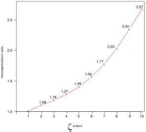
4.3.2 Homogenization ratio . . . 62
4.4 Discussion . . . 62
4.4.1 Biotic homogenization scenarios . . . 63
4.5 Conclusions . . . 66
4.6 Figures . . . 67
5 Comparison of clustering methods for pest prole analysis . . . 69
5.1 Introduction . . . 69
5.2 Methods . . . 71
5.2.1 Data . . . 71
5.2.2 Test design . . . 72
5.2.3 Clustering methods . . . 73
5.2.3.1 Self-organizing maps . . . 73
5.2.3.2 Self organizing maps for analysis of pest proles . . . 74
5.2.3.3 K-means . . . 74
5.2.3.4 K-means for analysis of pest proles . . . 75
5.2.3.5 Hierarchical clustering . . . 75
5.2.3.6 Hierarchical clustering for analysis of pest proles . . . 76
5.2.4 Evaluation methods . . . 76
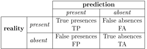
5.2.4.1 Confusion matrix and derived metrics . . . 76
5.2.4.2 ROC evaluation . . . 78
5.2.4.3 Overall performance metrics . . . 78
5.3 Results . . . 79
5.3.1 Distributions of risk indices per method . . . 79
5.3.2 Aggregate performance metrics . . . 81
5.3.3 Results by clustering method . . . 82
5.3.3.1 Control . . . 82
5.3.4 Hierarchical Clustering . . . 82
5.3.4.1 SOM . . . 82
5.3.5 K-means . . . 83
5.4 Map of the HC clusters . . . 83
5.5 Discussion . . . 84
5.5.1 Issues encountered . . . 84
5.5.2 Number of clusters and environmental lter hypotheses . . . 85
5.5.3 Performance metrics . . . 87
5.5.3.1 Comission and omission errors equal weights . . . 87
5.5.4 Choosing the best method . . . 88
5.5.5 Implications for PPA . . . 89
5.5.6 Perspectives and future research . . . 90
6 General Discussion . . . 93
6.1 Preamble . . . 93
6.2 Methodological improvements . . . 94
6.3 Model validation . . . 95
6.3.1 Operational validation tests . . . 95
6.3.2 Conceptual validation of ecological principles . . . 96
6.4 Final remarks . . . 99
A Supplement chapter 2 . . . A A.1 Weights variability . . . A A.2 Ranks variability . . . G A.3 Species prevalence . . . J A.4 Related publication . . . J
B Supplement chapter 3 . . . M B.1 Species area relationship . . . M B.2 Minimal working example of the computation ofζ . . . N
B.3 Richness . . . O
C Supplement chapter 4 . . . Q C.1 Computingζ . . . Q
C.2 Signicance test forζ values . . . R
List of Figures
1.1 Visualization of SOM input layer, output layer and its relationships. Adapted
from http://matias-ck.com/mlz/somz.html. . . 11
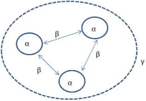
1.2 Conceptual plot of the α,β and γ diversities for three sites . . . 16
2.1 Diagram of SOM PPA process . . . 28
2.2 Details of datasets preparation and nomenclature . . . 29
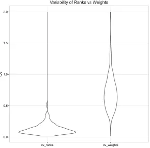
2.3 Comparison of CV density distribution for ranks and for weights . . . 33
3.1 Diagram of SOM PPA. Regions clustered in red neurons are more similar to the target region than regions clustered in green neurons . . . 45
3.2 ζdecline in SOM map neurons. (a) shows SOM map with some regions located according to their regional insect pest proles. (b) shows ζ1 (average species richness of all the regions clustered in a neuron). (c) corresponds to normalized ζ2 per neuron (average proportion of species any two regions in that neuron share). And (d,e,f) correspond respectively to normalized ζ3, normalized ζ4 and normalized ζ5 . . . 48
3.3 Scheme of the three levels of uncertainty for the output risk list that emerged from theζ values on the SOM output map . . . 51
4.1 Percentage increase of α for all the regions considered in the CABI CPC database from 2003 to 2014. Warmer colors indicate percentage decreases in α, yellow indicates no change in α and colder colors indicate percentage increases inα. . . 67
4.2 Plot of homogenization ratios calculated as a ratio of normalizedζ values for 2014 to normalizedζ values for 2003 . . . 68
5.2 ROC space plots for all the methods. Specicity values in Y axis and (1-Sensitivity) values in the X axis . . . 81
5.3 Map of the 4 clusters obtained by HC . . . 84
A.1 Histogram of weight values for 199 species . . . A
A.2 Boxplot of weight values for 199 species . . . B
A.3 Relationship between Mean and SD of weight values . . . C
A.4 Scatterplot of CV values for 199 species . . . D
A.5 Histogram of CV values . . . E
A.6 Boxplots of the weight value for 5 top and 5 bottom average weights species. Mid-line indicates median value and whiskers depict variability outside the upper and lower quartiles . . . F
A.7 Values of the R∗ for the subset of 199 species . . . G
A.8 Relationship between mean and SD of the R∗ value . . . H
A.9 Histogram of the values of the coecient of variation of the average rank R∗
for the subset of 199 species . . . I
A.10 Species prevalence plotted against species mean weight values. (log-log) . . . J
B.1 Species-Area relationship tted into a log-linear Gleason model. (k=−14.86, P r(>
|t|= 0.15;slope= 9.98, P r(>|t|= 2e−16)) . . . M
B.2 Sorensen values per neuron of the SOM output map . . . O
C.1 ζ values computed from randomly generated assemblages (dots) and ζ
val-ues computed for the observed data for each year (red lines). Y axes are in logarithmic scale. . . R
List of Tables
1.1 Denitions of the levels of invasiveness used in this thesis. Adapted from Blackburn et al. (2011) . . . 2
1.2 Uncertainty typologies from the literature - 1990 to 2008(Modied from As-cough et al. (2008)) . . . 18
2.1 SOM PPA terminology . . . 27
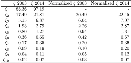
4.1 Columns 1 and 2 showζvalues for the 2003 and 2014 pest occurrence matrices,
units are species counts. Columns 3 and 4 show the average percent shared species between iassemblages, where iis the order ofζ. . . 62
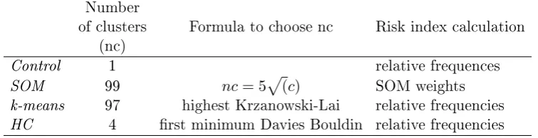
5.1 Summary table of tested methods and their specications . . . 73
5.2 Confusion matrix . . . 77
5.3 Summary statistics of risk indices per method and for 2014 observed data. Observed 2014 data are binary . . . 80
5.4 Aggregate (threshold-independent) performance metrics calculated for each method . . . 82
Chapter 1
General introduction
1.1 Biological invasions and Biosecurity
The book `The ecology of invasions of animals and plants' by Charles S. Elton in 1958 is considered to have set the basis of the Invasion Biology eld. It described the global distributions of seven invasive species and analysed, for the rst time, the relationships between the species' populations and the habitat patterns that were disrupted by them (Arnold B . Erickson, 1960).
Since then, invasive species have been considered by many sub-disciplines in ecol-ogy, biology and biogeography and, due to this multidisciplinarity (Hulme, 2011), they have also been the source of extensive debate. There have been two main groups of inva-sion biologists divided by the taxa they study; those concerned with animal invainva-sions and those concerned with plant invasions (Blackburn et al., 2011). Each of those groups has adopted dierent invasion model frameworks, resulting in controversy about the adequate-ness of the terminology and the limits of the concepts and denitions. Basically, animal ecologists traditionally have followed Williamson's invasion framework (see (Williamson, 1989; Williamson & Fitter, 1996; Williamson, 2006)) while plant ecologists have followed Richardson's classications (Richardson et al., 2000, 2011). Eort has recently been made (Blackburn et al., 2011) to bring together the animal and plant invasions ecology tradi-tions to create a general invasion ecology framework. Another notable dispute in invasion biology has concerned the political and ethical standpoints towards the invasive species problematic (see Warren (2007) for a critique of the language and practice in the eld, then Richardson, D.M., Py²ek, P., Simberlo, D., Rejmánek, M., Mader (2008) for the response and then Warren (2008) for the counter-response).
framework for biological invasions and dene an alien species as a non native species that has been transported beyond the limits of its native range by human mediated dispersal. The arrival of an alien species can result in dierent degrees of colonization. One widely accepted system to characterize the potential colonization success is the naturalization-invasion framework (Py²ek et al., 2004; Richardson & Py²ek, 2012) that excludes previous binary denitions of invasiveness. Instead, each alien species is placed somewhere along a continuum from casual invader to successful invader depending on the invasion stage (or barriers) that they have overcome. Nevertheless, it is also informative to dene degrees of invasiveness according to colonization success. (See Table 1.1.)
Table 1.1: Denitions of the levels of invasiveness used in this thesis. Adapted from Blackburn et al. (2011)
Level of invasiveness Denition
Casual Alien species transported out of its native range either in captivity or quarantine. When released into the novel environment it is incapable of surviving for a signicant period.
Naturalized/Established Alien species with individuals surviving in the wild in the location where they were introduced, either
reproducing or not. A wild population might be sustained. Invasive Alien species with self-sustaining populations at multiple sites
in the wild, with individuals spreading
signicantly from the original point of introduction.
Many ecological factors have been shown to inuence the success of alien invasions (Williamson, 2006). They have been summarized in Pimentel et al. (2005) as: 1) lack of natural enemies in the new habitat, 2) development of new host or parasite associations 3) presence or absence of other predators 4) degree of disturbance of the newly colonized habitat, and 5) degree of adaptability of the species. Much attention has also been paid to invasion consequences or impacts. An invasive species is likely to cause some impact that will alter the established order of the invaded ecosystem (Vitousek et al., 1996), and potentially stimulate some physical and structural changes in those ecosystems where it is introduced (Mack et al., 2000; Simberlo, 2011).
According to the International Union for Conservation of Nature (IUCN), a species is a pest if it causes either other species to decline or the structure and function of natural and productive ecosystems to be altered, resulting in economic impacts and/or decreases in biodiversity (IUCN/SSC, 2000; Worner, 1991). Therefore, in this thesis I follow IUCN criteria and dene a pest as an invasive species that can either cause economic damage or a decrease in biodiversity in the environment where it has been introduced.
1.1.1 Biosecurity: Policies, Agencies and Pest Risk Analysis
Modern societies depend on productive economies which rely on trade, market access and tourism. Together, global movements of people and goods facilitate the spread of pest species. Human assisted dispersal of pest species occurs through the direct imports and exports of commodities, and also as pests hitch-hiking in containers, other conveyances, and even on humans themselves. Regardless of entry pathway, the arrival of a pest causes a change to the recipient nation's economic well-being, due to both its arrival and to the eorts taken to mitigate its impact (Perrings et al., 2005; Warziniack et al., 2013).
Most trading nations have recognized the invasive species problem and have estab-lished regulated trade procedures to mitigate it. The United Nations' Food and Agri-culture Organization (FAO) and the World Trade Organization (WTO) have produced several worldwide agreements and standards, such as the International Plant Protection Convention (IPPC). The IPPC is an international agreement on plant health, currently with 180 adhering countries, which aims to protect cultivated and wild plants by prevent-ing the introduction and spread of plant pests. To support the IPPC, there are currently nine regional plant protection organizations (RPPOs) around the world. Some of these are the European and Mediterranean Plant Protection Organization (EPPO), the Inter-African Phytosanitary Council and the North American Plant Protection Organization (NAPPO) (all are listed in https://www.ippc.int/en/partners/regional-plant-protection-organizations/). Some countries also have their own national plant protection organisa-tions (NPPOs). Examples are New Zealand's biosecurity agency regulators within the New Zealand Ministry for Primary Industries and Australia Biosecurity within the Australian Department of Agriculture, Fisheries and Forestry. Those two agencies are commonly used as an example of what would be desirable elsewhere, mainly due to their rigorous management of phytosanitary risks from international trade (Bacon et al., 2012).
that cross the border each day (in New Zealand that number is estimated at 170,000 a day (Silcock & Guy, 2013)) biosecurity programs cannot target all alien species. Instead, border controls, policies and quarantine procedures have to be eciently prioritised and implemented.
To help achieve such eciencies, the IPPC published the International Standards for Phytosanitary measures (ISPMs), which are part of the FAO global programme of policy and technical assistance in plant quarantine. This programme makes available to FAO members and other interested parties, standards, guidelines and recommendations to achieve international harmonization of phytosanitary measures. Some interesting tools provided by the ISPMs are the general Phytosanitary principles for the protection of plants and the application of phytonsanitary measures in international trade (ISPM 01) (Interna-tional Plant Protection Convention (IPPC), 2006a), the Framework for pest risk analysis (ISPM 02) International Plant Protection Convention (IPPC) (2007) and the pest risk anal-ysis for quarantine pests (ISPM 11) (International Plant Protection Convention (IPPC), 2004). All the ISPMs were republished in 2016 and are publicly available at the FAOs website (https://www.ippc.int/en/core-activities/standards-setting/ispms/).
1.1.1.1 Pest Risk Analysis
Pest risk analysis (PRA) is divided into three stages: initialization, assessment of the risk, and management. During initialization, the pests and pathways that require PRA are identied. Then, pest risk assessment determines the status of each species as a pest, its associated entry pathways, and characterizes its likelihood of entry, establishment, spread and economic importance. The third stage; pest risk management, involves the development, evaluation, comparison and selection of strategies for reducing risk. The geographical area to which a PRA applies is usually a country, but can also be an area within a country, or a more extensive area covering all or parts of several countries.
data from global databases (see McGeoch et al. (2012) for a review of uncertainty present in invasive species listings) and interpret it, within restricted time frames, to extract the information needed for decision making. PRA are science-based evaluations that usually involve reviewing and interpreting articles and databases but not scientic experimenta-tion. Usually risk analysts draw on scientic literature to make inferences regarding the components of the overall risk(McLeod, 2015). Many quantitative and qualitative tools have potential to assist pest risk analysts with this complex process.
While academic research has focused on rening quantitative predictive models for risk assessment (some examples are (Liu et al., 2011; Singh et al., 2015; Wattenbach et al., 2006)), policy improvements have centred upon better elicitation of expert knowledge based on risk-scoring methods (Leung et al., 2012). Qualitative methods generally consist of subjective statements (often verbal classications) regarding elements contributing to risk before providing a conclusion on the overall risk (McLeod, 2015). However, expert-based risk assessment is known to be highly biased by the experts morals, beliefs and by their self-perceived objectivity (Burgman, 2005). On the other hand, quantitative methods aim to obtain numerical estimations of the risk, using deductive statistical approaches. However, quantitative models for PRA are often perceived as too complex and uncertain by pest risk analysts and can also be biased by subjective knowledge when data for risk factors are unavailable or uncertain (McLeod, 2015). Both quantitative and qualitative PRAs and their combinations can be improved, although it is unrealistic to expect a completely automatated quantitative method that makes expert input redundant and can be used under any circumstance for any pest (Sutherst & Bourne, 2008; Sutherst, 2014).
1.1.1.2 Quantitative approaches to PRA
re-quired in invasion biology (Lewinsohn et al., 2005; Chown, 2015), there is a biogeographic approach to pest risk assessment.
In general terms, quantitative biogeographical approaches to pest risk assessment (also known as `pest risk mapping' (Venette et al., 2010)) aim to prioritize geographic domains suitable for the establishment of pest species (insects, weeds or diseases). Pest risk mapping produces models, lists and maps that can help answer questions of what species are of concern, where these species occur, how they may spread if they were introduced and what their potential impacts might be. These models, maps and tools should have strong fundamental ecological and geographical foundations. Some reviews of biogeographical approaches to pest risk assessment can be found in Sutherst (2014) and Leung et al. (2012), along with model comparisons in Sutherst & Bourne (2008) and also a list of the identied aws and directions for improvement in Venette et al. (2010).
In this thesis I am interested in the subset of the quantitative biogeographical ap-proaches to pest risk assessment, specically the creation of lists of pest prioritization based on the study of global invasive pest assemblages.
1.2 Global invasive assemblages analyses
An assemblage of species is the group of species occupying a particular site. In the con-text of agricultural plant protection, the species of interest are crop pests, either insects, weeds or other pests and pathogens such as fungi, virus and bacteria. Therefore, the pest assemblage of a region is the group of pest species that co-occur in that region.
1.2.1 Pest prole analysis (PPA)
and potentially to other taxa. The authors used the terminology `pest prole' of a region as an exact synonym of `pest assemblage' of a region, and it has been since then used in-terchangeably across all related literature (Table of terminology and synonyms in Chapter 2, section 2.1).
The rationale behind pest prole analysis is that a pest assemblage implicitly con-tains information about a region's biotic and abiotic conditions. Biotic conditions that can inuence the composition of the assemblage inlcude, for example, the agricultural crops grown in the region and inuential abiotic conditions include the region's climatic charac-teristics (Eyre et al., 2012). Other regional characcharac-teristics that could inuence assemblages include the tectonic activity, historical trade paths (Ricklefs, 2004), structure and quantity of trade, and the biosecurity measures applied. It is assumed that regions with similar pest proles will also have similar biotic and abiotic characteristics that allow the species to establish. Therefore, comparing pest assemblages between regions can provide insights about which regions may exchange species with high probabilities of establishment.
Worner & Gevrey (2006) and Gevrey et al. (2006) analysed pest assemblages using a clustering method known as self-organizing map (SOM) (Kohonen, 1982, 1990). Section 1.2.2.1 contains a more detailed introduction to the SOM algorithm. The SOM method is especially useful for clustering highly dimensional data and has been be applied to many elds of scientic research (see Oja et al. (2003) for a detailed review of applications), such as nance (Deboeck & Kohonen, 1998), genomics (Törönen et al., 1999), natural language processing (Honkela, 1997) and numerous areas of ecological sciences (Chon, 2011) where it has successfully described environmental or species spaces by clustering sets of environmental variables.
plant parasitic nematodes, and Singh et al. (2015) incorporated the PPA approach into a quantitative PRA method called pest screening and targeting (PeST). Broader extensions were also made by Morin et al. (2013) who applied PPA for the rst time to studying and prioritizing of weeds and by Eschen et al. (2014) who applied it to assemblages of bacteria and nematode pests.
1.2.2 Methodological approaches to PPA
Clustering is the process through which the data is divided into meaningful groups and it is usually one of the rst steps in analysing data (Davies & Bouldin, 1979). The aim of clustering is partitioning the data into groups such that the observations in a cluster (group) are more similar to each other than observations in dierent clusters (Mangiameli et al., 1996). In cluster analyses, there are no predened classications and the clustering algorithm has the task to divide the data into natural groups. Algorithms that perform clustering are called unsupervised learning algorithms.
1.2.2.1 Introduction to Self-Organizing maps
A self-organizing map (SOM) is an algorithm that belongs to the family of articial neural networks. It is an information-processing paradigm inspired by the functioning of verte-brate brains (Kohonen, 2013). A SOM neural network is composed of two layers of neurons: the input layer and the output layer. Let the data be organized in a matrix where the rows are the input patterns (observations) and the columns are the input neurons (variables). The output layer is represented by a rectangular grid withm∗nneurons (also called cells
times as the number of epochs. Each neuron of the input layer, has as many weights as the input patterns, and can thus be regarded as a vector in the same space as the patterns.
Output neurons are initialized randomly (are given a set of coordinates (weights) in the multidimensional output space) and then they are trained. When the SOM is trained to an input pattern, the distance between that specic pattern and every neuron in the output space is calculated. Then the closest neuron in terms of distance (Euclidean distance) is dened as the winning neuron, and the pattern is mapped onto that winning neuron. As a consequence, the neuron moves toward the input pattern position in order to improve its representation and this movement is translated into a change in its coordinates (weights). The extent of this movement is controlled by a parameter usually referred to as learning rate.
In order to preserve the topology of the input patterns in the output space, it is essential to correct both the position of the wining neuron and also the position of its neighbouring neurons. Thus, the network is progressively organized (unfolded) with certain parts of the input space being represented by certain subsets of neighbouring neurons. The rst part of the training phase is the coarse training or unfolding, where the neurons of the output space are spread out and pulled towards a general area of the multidimensional space, thus dening its general shape. The second is the ne tuning phase, where the SOM matches the neurons as far as possible to the input patterns, thus decreasing the quantitization error.
If a SOM has been successfully trained, then patterns that are close in the input space will be mapped to neurons that are close (or the same) in the output space. This quality is called topology preserving.
is an unsupervised learning algorithm rst described in MacQueen (1967) that produces crisp clusters through a partitional clustering procedure. Partitional clustering attempts to directly decompose the data into a set of unrelated clusters by attempting to determine an integer number of partitions that optimise a certain criterion function (Halkidi et al., 2001). The procedure follows a simple and easy way to classify a given data set through a certain number of clusters (assume kclusters) xed a priori. The main idea is to dene
k centroids, one for each cluster. K-means clustering aims to partition n observations
into k clusters in which each observation belongs to the cluster with the nearest mean,
serving as a prototype of the cluster. The cluster centroids are initialized by placing them as far as possible from each other. Then, each input pattern is associated to its nearest centroid. When all the input patterns have been associated, the rst step is completed and an early grouping is done. At this pointk new centroids are recalculated. After these
k new centroids are obtained, a new binding has to be done between the same data set points and the nearest new centroid, as a result the k centroids change their location step by step until no more changes occur.
The algorithm proceeds (Adapted from Watts & Worner (2009)):
1. Select k seeds as initial centroids. These can be vectors that are generated randomly,
or vectors that are selected from the data set being clustered. 2. Calculate the distance from each cluster centroid to each seed. 3. Assign each observation to the nearest cluster.
4. Calculate new cluster centroids, where each new centroid is the mean of all vectors in that cluster.
5. Repeat steps 2 to 4 until a stopping condition is reached.
A key assumption of k-means is that the algorithm expects the data clusters to be spherical and of same size, so that the assignment to the nearest cluster center is the correct assignment.
1.2.2.3 Introduction to Hierarchical clustering methods
by either merging smaller clusters into larger ones, or by splitting larger clusters. The result of the algorithm is a tree of clusters, called dendrogram, which shows how the clusters are related. By cutting the dendrogram at a desired level, a clustering of the data items into disjoint groups is obtained (Halkidi et al., 2001).
There are many variations of hierarchical clustering algorithms, and they can be roughly divided into:
Agglomerative. These step-wise algorithms merge results from the previous step by merg-ing the two closest clusters into one.
Divisive. These step-wise algorithms split results from the previous step by splitting a cluster into two.
1.3 Global invasive assemblage diversity
Community ecology studies the diversity, abundance and composition of species in commu-nities. Traditionally it focused on the processes that determine the species composition of local communities but eventually recognised that the composition and diversity of species, even at a local scale, depended fundamentally on the composition and diversity of the regional pool of species (Vellend, 2010). The species pool is a concept rooted in island bio-geography and refers to all the species that are able to disperse to a focal site, regardless of their ability to tolerate the site's environmental conditions (Cornell & Harrison, 2014). The environmental lter is the relationship between a species and the environment, which acts as a selective force by ruling out species that are unable to tolerate particular environ-mental conditions. Species that are able to survive at a site may have certain phenotypic traits that reect their environmental tolerance, and these traits may be shared among other species in the community. Consequently, species at a site exhibit phenotypic con-vergence in key ecological dimensions compared to a null expectation based on randomly sampling species from the larger species pool (Kraft et al., 2014).
ran-dom changes in species abundances (drift) and ongoing dispersal (Vellend, 2010). Thus, community assembly is inuenced by processes operating at a wide range of spatiotem-poral scales, and local communities are assumed to reect the cumulative eects of these processes (HilleRisLambers et al., 2012).
1.3.1 Diversity of herbivore insect assemblages
The global compositional variation of non-native regional insect assemblages has been shown to dier from the global compositional variation of native insect assemblages by Liebhold et al. (2016), who also noted that the invasive species compositions dier from what would be expected from island biogiography predictions (Liebhold et al., 2016; Burns, 2015). This suggests strong eects of human mediated dispersal and entry pathways.
For insect crop pests, the history of invasions is intimately linked to the history of agriculture. Crop pest regional assemblages are strongly correlated with the distribution of their host plants (Bebber et al., 2014a), which in turn may also be related to the climate suitability of the region (Bacon et al., 2014; Baker et al., 2005).
Agricultural landscapes are highly disturbed. As Pimentel et al. (2005) noted, 90% of the food consumed by humans is being provided by only fteen plant species. Conse-quently, agricultural landscapes across the world are very homogenized and environmental and ecological dierences between cultivated regions in dierent parts of the world have been greatly reduced. When a crop pest is introduced to a new and remote area, the expected mismatch between its phenotypic characteristics and the local ecological condi-tions expected to act as an environmental lter, have been greatly attenuated (Guillemaud et al., 2011).
1.3.2 Biotic Homogenization of crop pest assemblages
Biotic homogenization (Vitousek et al., 1996; McKinney & Lockwood, 1999; Lockwood & McKinney, 2001) is the phenomena through which the ongoing arrival of non-native species and the habitat disturbance caused by agricultural human practices (Vellend, 2010) increases the spatial and temporal similarity in the taxonomic composition of global biota. The immediate consequence of biotic homogenization is global loss of biodiversity.
Olden & Po (2003) noted empirical studies of biotic homogeneity were increasing, but there were knowledge gaps in its theoretical aspects, thus they drafted a rst conceptual model that comprised 14 theoretical ecological scenarios and mechanisms through which species invasions and extinctions led to dierent trajectories of biotic homogenization. Olden (2006) emphasized the lack of studies that examined and quantied the homoge-nization process for communities at multiple spatial and temporal scales. Many studies have found evidence of biotic homogenization and its links to agriculture for local commu-nitites, sometimes to the larger extents of countries or regions. For example, Vellend et al. (2007) found homogenization patterns in forest plant communities in North America and Europe due to agricultural land use and (Kuussaari et al., 2010) reported a decrease in diversity of butteries in intensively cultivated landscapes with simplied land structure. However, Olden & Po (2003) also reported some studies that questioned the existence of biotic homogenization. An example was Marchetti et al. (2006) on community composi-tion of freshwater sh communities in California which reported biotic dierentiacomposi-tion, or an increase in community diversity after the introduction of exotic species.
To our knowledge, two studies have measured biotic homogenization at a global extent. Bebber et al.(2014a) studied the distributional changes of 424 crop pests and pathogens over the years 2000 to 2014, and McKinney (2004) studied the plant inventories of 20 localities in the United States to measure whether exotic plants increased the simi-larity of those localities. Both Bebber et al. (2014a) and McKinney (2004) concluded that when considering exotic species only, their data showed signs of biotic homogenization.
their compositional β diversity.
1.3.2.1 Measures of diversity
Beta diversity encompasses a variety of indices and concepts that reect dierent compo-nents of between-sites species variability, or species turnover along environmental, spatial or temporal gradient (Whittaker, 1972; Vellend, 2001). There is a huge variety of indices that measure species richness at a spatial level, most of which represent slightly dier-ent natural phenomena (Tuomisto, 2010), therefore it is important to clearly dene for any particular study the expression used to calculate alpha, beta and gamma diversity (Anderson et al., 2011).
In this thesis we refer toβdiversity as species compositional variation between sites,
α diversity as the number of dierent species occurring at one site, and γ diversity as the
number of dierent species in the regional species pool (Whittaker, 1972), (Figure 1.2).
Figure 1.2: Conceptual plot of the α,βandγdiversities for three sites
Two problems associated withβ diversity metrics are that community pairwise
Thus, when such metrics are used to compare larger groups, they are calculated by averag-ing the pairwise metrics across sites. To circumvent these issues, Hui & McGeoch (2014) proposed the zeta diversity (ζ) metric. Zeta diversity (ζ) is a measure of compositional
β diversity dened as the number of species shared between any inumber of sites or
as-semblages. Zeta is a simple similarity measurement that reconciles existing descriptors of species incidence and spatial turnover (Hui & McGeoch, 2014) and overcomes the main crit-icisms posed against the pairwise similarity measures such as Jaccard, Sorensen (Sørensen, 1948) and Shannon (Shannon, 1948). The ζ metric is unaected by site-dependence, and
enables more than two sites to be compared at once. This multi-site comparison feature allows dierent orders (numbers of features compared at at time) of ζ to describe dierent
levels of similarity that can be very useful to understand the relationship between groups. In this thesis I use the metric ζ as the standard measure of αand β diversity.
1.4 Uncertainty in Ecological Modelling
1.4.1 Model based decision frameworks
char-Reference from literature Types of uncertainty considered (United States Environmental
Protection Agency, 1997) Scenario uncertainty, parameter uncertainty,model uncertainty (Morgan & Henrion, 1990),
(Hof-stetter, 1998) Statistical variation, subjective judgement,linguistic imprecision, intherent randomness disagreement, approximation
(Funtowicz & Ravetz, 1990) Data uncertainty, model uncertainty, com-pleteness uncertainty
(Bedfort & Cooke, 2001) Aleatory uncertainty, epistemic uncertainty, parameter uncertainty, data uncertainty, model uncertainty, ambiguity, volitional un-certainty
(Huijbregts et al., 2001) Parameter uncertainty, model uncertainty, un-certainty due to choices, spatial variabil-ity, temporal variabilvariabil-ity, variability between sources and objects
(Bevington & Robinson, 2002) Systematic errors, random errors
(Regan et al., 2002) Epistemic uncertainty, linguistic uncertainty (Walker et al., 2003) Location: context uncertainty, model
uncer-tainty, level uncertainty
(Maier et al., 2008) Data uncertainty, model uncertainty, human uncertainty
Table 1.2: Uncertainty typologies from the literature - 1990 to 2008(Modied from Ascough et al. (2008))
acterize the potential uncertainty in model-based decision processes, and it can be used to assess uncertainty in the same fashion as sensitivity (Matott et al., 2009). Drawing from Walker et al. (2003) 's framework, Wattenbach et al. (2006) developed a specic decision making process framework applied to ecosystem models.
Clearly, one of the biggest challenges in assessing uncertainty in any kind of ecolog-ical or environmental modelling is homogenizing the terms and concepts (Uusitalo et al., 2015a; Aggarwal, 2009). Dierent taxonomies of uncertainty have been framed by dier-ent authors, and the confusion is great. The work published by Ascough et al. (2008) brought together most of the research regarding uncertainty in environmental decision-making processes and summarized all these dierent denitions in a comprehensive table (Table 1.2).
and wordings; and decision uncertainty which is very important and is frequently under-estimated by the policy assessors. There are also categories of uncertainty that are not reducible and arise from sources that we have no control of. It can also be called random or stochastic uncertainty and is related to the chaotic and unpredictable quality of natural and social processes.
1.4.2 Reducing versus showing uncertainty
Two strategies can be adopted when dealing with uncertainty from a modelling point of view: reducing uncertainty whenever possible and showing uncertainty whenever it is ir-reducible. For implementing both strategies and for reducing uncertainty, they are highly case specic. A detailed review of methods for assessing uncertainty in predictive methods can be found in Lustig (2016). For showing irreducible uncertainty, a standard framework has been prepared in the form of an ISO document (Joint Committee for Guides in Metrol-ogy (JCGM), 2008) in which clear guidelines are given on how to express magnitudes and measurements that contain aleatory uncertainty.
1.5 Research questions and objectives of this thesis
There is a need for quantitative approaches to help the decision making process in the context of pest risk analyses. In this introductory chapter I presented the current state of existing models for pest prole analysis, and the conceptual ecological principles and theories behind the study of regional pest assemblages. I also reviewed current approaches to incorporating uncertainty in modelling to assist decision-making. However, some of these areas need further study, development and validation.
1.5.1 Validation and methodological improvements for PPA
choosing the number of clusters (Mirkin, 2013) and validating the clustering results (Halkidi et al., 2001).
To validate clustering results, they would ideally be compared to reality, but often the required information is either unavailable or insucient to both train and validate the models. A common solution is to validate using articially created, error-free data (Zurell et al., 2010). For SOM PPA this sort of validation was carried by Paini et al. (2011) by simulating a virtual world with several invasibility parameters for its regions, and the comparing the SOM PPA rankings to those of the nal invasions of the species. However, it is necessary to test the performance of the method against real observed values. Thus, we propose to carry out a model validation for SOM PPA using real occurrence data and compare the predictions of the model to the observed real values.
The SOM algorithm has advantages compared with the other main classication techniques of k-means and hierarchical clustering (HC) that make it particularly useful for analysing ecological data. Its biggest asset is the ability to capture non-linear rela-tionships. Non-linear relationships between observations and variables will often occur in highly dimensional datasets which means some variables will be irrelevant or redundant, and present outlier observations (Mangiameli et al., 1996; Park et al., 2003) However, it is uncertain if SOMs are always the best clustering method for ecological data. Watts & Worner (2009) compared the SOM PPA to k-means algorithm and it seemed k-means per-formed better, both computationally and quantitatively. Other research studies have used other clustering algorithms such as hierarchical clustering (Eschen et al., 2014) to perform PPA. It is my aim to understand which of these three clustering methods performs better with data such as global pest proles.
Besides problems relevant to all clustering methods, some specic issues of SOMs have been identied by recent work. They can be summarized as: 1) when global prevalence of a species is small, the SOM PPA apparently is not very accurate at generating good rankings for the species (Singh et al., 2013) 2) regions with pest proles comprising fewer than eight species are signicantly more unstable or dicult to predict (Paini et al., 2011) 3) the analysis can be aected by sampling artefacts; and 4) direct comparison of risk levels between dierent databases may not be possible (Worner et al. unpublished).
measure of `goodness' or uncertainty, and it would benet from a measure of uncertainty to better communicate its results to its intended end user, the risk assessor.
1.5.2 Study of the compositional diversity of regional pest assemblages
The PPA methodology is based on fundamental ecological principles such as the assemblage composition and the drivers behind community assembly. The main ecological hypothesis behind PPA is that two regions with similar pest proles share environmental and historical conditions that enable them able to support similar assemblage of pest species. Therefore, identifying similar regions may help to identify regions that are most likely to succesfully exchange pest species in the future, which would assist pest risk assessment.
This hypothesis is based on robust community ecology principles, but remains em-pirically untested. In this research I explored the composition of global pests assemblages in terms of composition and diversity and describe their changes over time. By quantifying their levels of biotic homogenization in this way, I aim to better describe the ecological assembly mechanisms on which the PPA hypothesis is based.
1.5.3 Specic objectives
Objective 1: To perform a sensitivity analysis of SOM PPA in order to clarify the issues that other authors have found when using the method.
Objective 2: To validate the SOM PPA outputs by explaining results of the clustering process through the lens of community assembly.
Objective 3: To compare the performance of dierent clustering methods for PPA and nd which method performs best according to the nature of the data.
Objective 4: To test the validity of inferring risks of invasion from clustering of pest proles.
1.6 Thesis structure
1.6.1 Chapter 2: Sensitivity analyses of SOM PPA
Chapter 2 examines how variation between datasets inuences the ouptuts of SOM PPA. The validity of using SOM weights and SOM ranks (model outputs) is tested by applying SOM PPA to 341 datasets and assessing the variability of its outputs.
1.6.2 Chapter 3: Cluster validity and uncertainty assessment of SOM PPA
Chapter 3 explores the value of incorporating an extra step in the SOM PPA method which consists of calculating a cluster validation metric (ζ diversity) that assesses the goodness
of cluster of the SOM PPA results. It also proposes the zeta diversity metric as a measure of uncertainty communication for SOM PPA.
1.6.3 Chapter 4: Calculating the degree of Biotic Homogenization for PPA
Chapter 4 analyses the degree of homogenization among global insect pest proles. The analysis compares the degree of similarity between regional pest proles in two dierent years and uses ζ diversity as a new measure of quantication of biotic homogenization.
1.6.4 Chapter 5: The informative power of clustering pest proles: Comparison of methods
Chapter 5 evaluates the PPA predictive power and a comparison of clustering methods. Three dierent clustering approaches (SOM, k-means and hierarchical clustering) are ap-plied to a global dataset of pest occurrences in the year 2006 and then validated with an equivalent dataset that documents the same pests' distributions observed in year 2014.
1.6.5 Chapter 6: General discussion
Chapter 2
Self-organizing maps for analysing pest proles:
Sen-sitivity analysis of weights and ranks
Notes
This chapter is published as:
Roigé, M., Parry, M., Phillips, C., Worner, S.P (2016). Self-organizing maps for analysing pest proles: Sensitivity analysis of weights and ranks, Ecological Modelling, 342, 113-122.
Abstract
Self organizing maps for pest prole analysis (SOM PPA) is a quantitative ltering tool aimed to assist pest risk analysis. The main SOM PPA outputs used by risk analysts are species weights and species ranks. We investigated the sensitivity of SOM PPA to changes in input data. Variations in SOM PPA species weights and ranks were examined by creating datasets of dierent sizes and running numerous SOM PPA analyses. The results showed that species ranks are much less inuenced by variations in dataset size than species weights. The results showed SOM PPA should be suitable for studying small datasets restricted to only a few species. Also, the results indicated that minor data pre-processing is needed before analyses, which has the dual benets of reducing analysis time and modeller-induced bias.
Keywords
2.1 Introduction
Over recent decades there has been considerable research on biological invasions and their impacts (Barlow & Goldson, 2002; Blackburn et al., 2014; Hulme, 2003; McGeoch et al., 2006). Such interest has caused invasion ecology to become a multidisciplinary eld, bring-ing together fundamental ecology, conservation, environmental management, border con-trol and biosecurity (Kolar & Lodge, 2001; Perrings et al., 2005; Vitousek, 1990). Despite its diversity, there is consensus about the need to develop proactive invasion prevention strategies rather than reactive pest management programs.
An important tool for preventing invasions is pest risk analysis, which draws together several sub-disciplines of quantitative and qualitative science. In most developed countries, biosecurity and quarantine agencies use pest risk analysis to help make decisions about which species and entry pathways to regulate (EPPO, 2004; International Plant Protection Convention (IPPC), 2006b; Leung et al., 2012).
Self-Organizing Maps for Pest Prole Analysis (SOM PPA) is a quantitative method intended to assist pest risk analysis, which was rst described by Worner and Gevrey (2006). A pest prole is the assemblage of insect pest species in a region, and a SOM is an articial neural network algorithm that performs unsupervised classication (Kohonen, 1982). In SOM PPA, pest proles for all geopolitical regions of the world are collected and their similarity is analysed. Regional proles clustered together are assumed to share similar biotic and abiotic conditions that have allowed their respective species assemblages to become established. The output of SOM PPA is a list of species ranked according to the level of the risk they present to the region under consideration. A species that is present in many of the regions which cluster with the target region but is absent for the target region, could establish in the target region if introduced. The level of risk is indicated by SOM species weights, which are explained below.
to 20%. Paini et al. (2010b) showed the predictive value of SOM PPA when applied to a simulated dataset.
Nevertheless, issues about using SOM PPA remain (Worner et al., 2013). SOM PPA uses weights as a proxy for species risk of establishment, but directly comparing SOM weights for the same species between studies is invalid because weight values change whenever dierent input data are used. This variability casts doubt upon the capability of SOM species weights to be used as indicators of species establishment risk. Weights change because they are m-dimensional coordinates in the m-dimensional space (where m is the
number of species) created by the SOM algorithm. Thus, when input datasets contain dierent species, the m-dimensional spaces and coordinates will also dier, and the same
species will receive dierent weights for the same target region. An alternative is to use species' relative ranks to generate the output risk lists (Paini et al., 2010b). However, it remains uncertain if relative ranks generally show more stability between input datasets than species weights.
An example can help explain the weights variability problem. In Worner and Gevrey (2006), the highest ranked species (rank 1) was Planococcus citri, which received a SOM weight of 0.93. The second ranked species (rank 2) was Icera purchase which had weight 0.92. When the analysis was run with updated data from 2014 (unpublished data), the global distributions of some species had changed, and Planococcus citri obtained a weight of 0.82 and Icera purchase obtained 0.71. Nevertheless, their ranks remained rst and second.
the input dataset represents a new dimension for the algorithm to account for, but also provides more information for the algorithm to learn from. Thus, there may be trade-os between number of species and the accuracy of SOM weights and ranks. Knight et al. (2011) tentatively explored the eects of data dimensionality (number of species) on SOM PPA results and obtained contradictory results.
The overall aim of our study was to investigate the sensitivity of the SOM PPA outputs to changes in input data. Specic objectives were to assess: the relationship between weight variability and number of species in the dataset, the relative stability of weights and ranks, and the relationship between weight, rank and global species prevalence. We created datasets of dierent dimensionality and studied changes in weights and ranks of each species.
2.2 Methods
2.2.1 Terminology
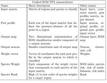
SOM PPA terminology is sometimes confusing. In table 2.1 we aggregated model nomen-clature used across the dierent studies cited in this paper, and chose one name for each feature.
2.2.2 The self-organizing map algorithm
Table 2.1: SOM PPA terminology
Unied SOM PPA nomenclature
Name Short description Other names
Input matrix Matrix of regions and species to classify Input layer, ocur-rence matrix, pest proles matrix, in-put dataset
Pest prole Each row of the input matrix that de-nes the presence/absence of all the pests in a region
Input neuron, gional prole, re-gional pest prole, input vector Output map Two dimensional representation of
SOM classication results composed of
noutput neurons
Output layer, SOM map
Output neuron Smaller constituent unit of output map Neuron, cluster, unit, cell
Weight vector Vector of coordinates for each pest pro-le in the output neuron to which is classied
Weights
Species Weight Each component of the weight vector that corresponds to each species of the input matrix
SOM index, species risk, risk of estab-lishment, risk index Species Rank High (1) to low order of species weights
for a target region Rank
2.2.3 The SOM PPA
In SOM PPA, rows of the occurrence matrix are regional pest proles. In the nal output map classication, two pest proles mapped to nearby neurons are more similar than two pest proles allocated to neurons that are far apart. Input and output neurons are linked through a parameter called the weight vector.
Weights describe the position in the output map of each of the regional proles of the input matrix. They are coordinates of each pest prole inm-dimensional output space
wherem is the number of species of the input matrix (Gevrey et al., 2006).
Ecologically, weights are interpreted as the degree of association between a species and a particular regional prole. Thus, the higher the weight for a species, the more closely associated the species is with that regional prole, and consequently, with all the regional proles clustered nearby. When modelling binary presence/absence data, weights range between 0 and 1.
datasetA 𝐵𝑎𝑝𝑝𝑙𝑒𝑠 𝐵𝑏𝑎𝑛𝑎𝑛𝑎𝑠 𝐵𝑐𝑜𝑡𝑡𝑜𝑛 𝐵𝑔𝑟𝑎𝑝𝑒𝑠 𝐵𝑚𝑎𝑖𝑧𝑒 𝐵𝑚𝑎𝑛𝑔𝑜 𝐵𝑝𝑜𝑡𝑎𝑡𝑜 𝐵𝑟𝑖𝑐𝑒 𝐵𝑡𝑜𝑚𝑎𝑡𝑜 𝐵𝑤ℎ𝑒𝑎𝑡 datasets 𝐵𝑖;𝑖=𝑐𝑟𝑜𝑝
460x 873
(regions x species) 460 x 35 460 x 33 460 x 34 460 x 46 460 x 60 460 x 30 460 x 35 460 x 52 460 x 36 460 x 38
460 x 10 460 x 10 460 x 10 460 x 10 460 x 10 460 x 10 460 x 10 460 x 10 460 x 10 460 x 10
460 x 20 460 x 20 460 x 20 460 x 20 460 x 20 460 x 20 460 x 20 460 x 20 460 x 20 460 x 20
460 x 30 460 x 30 460 x 30 460 x 30 460 x 30 460 x 30 460 x 30 460 x 30 460 x 30 460 x 30
𝐵𝑖10
(110 datasets)
𝐵𝑖20
(110 datasets)
𝐵𝑖30
(110 datasets)
Figure 2.2: Details of datasets preparation and nomenclature
We named these crop restricted matricesdatasetsBi, where i = crop(Figure 2.2).
The species present in each data set varied according to whether they were associated with the crop and associations were determined using the information in PQR. The range in the number of species in datasets datasetsBi was from 33 to 60 species. Finally, for each
crop-restricted matrix, we created 33 species restricted matrices through random sampling. Thus, for every datasetBi we created 11datasetBi10, 11datasetBi20and 11 datasetBi30, where 10, 20 and 30 are the number of species in each, j. The result was a total of 341
datasets (dataset A+ 10 datasetsBi+ 10∗33 datasetsBij). All data subsets contained
2.2.5 Weights sensitivity
To investigate the sensitivity of species weights and ranks to data dimensionality, we ran a complete SOM PPA for each of the 341 datasets for one target region (New Zealand) and created a ranked list of species from each run. The SOM initialization parameters were: 108 output neurons as given by the formulac= 5p(n)(Vesanto & Alhoniemi, 2000) wherecis
number of output neurons and nis number of training samples; Gaussian neighbourhood
distribution; linear initialization to ensure proper unfolding; and batch training mode as opposed to sequential training. The software used was SOM Toolbox (Vesanto et al., 2000) for Matlab R2013b (Mathworks, 2013).
We recorded the weight obtained for each species across the 341 SOM PPA. Since not all species occurred in all datasets, we selected 199 species out of the 873 that were each present in 10 or more of the 341 datasets. Because the datasets were created using random sampling, these 199 species comprised an unbiased sample of the total 873. To examine variability of species weights, we calculated descriptive statistics for the 199 species and conducted a graphical exploratory analyses for each. We used R (R Foundation for Statistical Computing, 2014) for statistical tests and data handling.
2.2.5.1 Weights variability
Univariant descriptive statistics were calculated to summarize the central tendency and the variability a of the weight values for each of the 199 species. Boxplots of weights were generated for each species.
2.2.5.2 Weights sensitivity to dataset size
2.2.6 Ranks sensitivity
To evaluate the sensitivity of species ranks to changes in dataset size we analysed their average rankR∗ and assessed its variability by computing some dispersion metrics such as
their standard deviations and coecients of variation.
2.2.7 Relationship between weight and species prevalence
We dened prevalence as the number of regions where a species was present. We graphically explored the relationship between prevalence and weight value for a single target region, and performed a linear regression to model the relationship. We expected to nd that species with higher worldwide prevalence would generally have higher weights (Singh et al., 2013).
2.3 Results
2.3.1 Weights sensitivity
2.3.1.1 Species weight variability between crop-restricted datasets containing dierent number of species
Across all species and crops, the mean weight was 0.137 and the median was of 0.024, which indicated a right skewed distribution (see histogram of weight values in A.1). Weight standard deviation was inadequate for measuring variability because it had a parabolic re-lationship with the mean (Figure A.3). This was unsurprising since weights are constrained between 0 and 1, thus their SD is less near the limits of their range values than in the middle.
2.3.1.2 Species weights sensitivity to datasets of dierent sizes
The linear mixed eects analysis of the relationship between weight and number of species showed weight was inuenced by dataset size (χ2 = 4.08, p-value = 0.0432), with each
additional species increasing it by 0.00002. The intra-species variability of the eect was of 0.2 SD. Species with low average weights showed less variation between datasets of dierent sizes than species with high average weights.
2.3.2 Ranks sensitivity
2.3.2.1 Species rank variability between crop-restricted datasets containing diering number of species
Many species occurred in few datasets, which made measurements of variation between ranks for these species uninformative. Thus, a subset of 674 species that had less than 10 appearances each across the 341 datasets (in other words less than 10 ranks) were excluded from the analysis. We studied average rank R∗ variability for the remaining 199 species
that occurred in ten or more datasets (as for weights).
Ranks for a given species usually varied between datasets. Average ranks were nor-mally distributed (Shapiro-Wilk normality test: W= 0.9745, p-value<0.0001, gure A.7),
ranged from 24.88 to 869.40 and had a mean of 460.
As for weights, CV was used to measure variation in average rank because SD had a parabolic relationship with the mean (gure A.8 cf. gure A.3). Of 199 species, 91 had CV <10%, 168 had CV <20%, and only two species had CV >50% (A.9).
Ranks were clearly less variable than weights, with lower CV. Figure 2.3 shows how their respective CV density functions dier.
2.3.3 Species prevalence
0.0 0.5 1.0 1.5 2.0
cv_ranks cv_weights
CV
Variability of Ranks vs Weights
Figure 2.3: Comparison of CV density distribution for ranks and for weights
against weight exhibited no relationship, even after applying logarithmic transformations to the data (Figure A.10). Linear regression also showed no signicant relationship (F-statistic 0.1893 on 1 and 871 DF, p-value=0.6636). This indicated that species ranked highly for the target region (New Zealand) were not necessarily those with the largest geographical distributions.