https://doi.org/10.5194/os-14-1523-2018 © Author(s) 2018. This work is distributed under the Creative Commons Attribution 4.0 License.
Parameterization of phytoplankton spectral absorption coefficients
in the Baltic Sea: general, monthly and two-component variants of
approximation formulas
Justyna Meler, Sławomir B. Wo´zniak, Joanna Sto ´n-Egiert, and Bogdan Wo´zniak
Institute of Oceanology, Polish Academy of Sciences, Powsta´nców Warszawy 55, 81-712 Sopot, Poland
Correspondence:Justyna Meler ([email protected]) Received: 14 June 2018 – Discussion started: 9 July 2018
Revised: 21 November 2018 – Accepted: 23 November 2018 – Published: 11 December 2018
Abstract. This paper presents approximate formulas (em-pirical equations) for parameterizing the coefficient of light absorption by phytoplankton aph(λ) in Baltic Sea surface waters. Over a thousand absorption spectra (in the 350– 750 nm range), recorded during 9 years of research carried out in different months of the year and in various regions of the southern and central Baltic, were used to derive these parameterizations. The empirical material was characterized by a wide range of variability: the total chlorophyll a con-centration (Tchl a) varied between 0.31 and 142 mg m−3, the ratio of the sum of all accessory pigment concentrations to chlorophyll a (P
Ci/Tchla) ranged between 0.21 and
1.5, and the absorption coefficients aph(λ) at individual light wavelengths varied over almost 3 orders of magnitude. Different versions of the parameterization formulas were derived on the basis of these data: a one-component param-eterization in the “classic” form of a power function with Tchla as the only variable and a two-component formula – the product of the power and exponential functions – with TchlaandP
Ci/Tchlaas variables. We found distinct
dif-ferences between the general version of the one-component parameterization and its variants derived for individual months of the year. In contrast to the general variant of parameterization, the new two-component variant takes account of the variability of pigment composition occurring throughout the year in Baltic phytoplankton populations.
1 Introduction
If we wish to fully describe the process of photosynthesis in the seas and oceans and to correctly interpret remote ob-servations of water bodies, it is important to obtain an ac-curate quantitative description of the spectral characteristics of light absorption by living phytoplankton, a significant con-stituent of seawater (e.g. Kirk, 1994; Mobley, 1994; Wo´zniak and Dera, 2007). The efficiency of sunlight absorption by this phytoplankton generally depends on a number of factors. The major, strongly absorbing components of phytoplankton cells are the pigments they contain. The principal photosynthetic pigment is chlorophylla, which absorbs visible light mainly in two bands: one situated in the blue region, with a maxi-mum around 440 nm, and another one in the red, with a max-imum around 675 nm (e.g. Bidigare et al., 1990; Bricaud et al., 2004; Wo´zniak and Dera, 2007). There are also various accessory pigments, like chlorophyllsb andc, carotenoids, and phycobilins. These latter pigments have different spec-tral absorption characteristics and may be involved in pho-tosynthetic, photoprotective or other processes in marine or-ganisms. The pigment composition of photosynthesizing ma-rine species can differ, since it can in a general sense re-flect the adaptation of an organism to different light condi-tions (photo- and chromatic adaptation) as well as acclima-tion at the plant community level (e.g. Kirk, 1994; Wo´zniak and Dera, 2007). Overall, analysis of pigment composition data obtained for marine phytoplankton assemblages from various ocean and sea waters has revealed a general trend indicating that the proportion of accessory pigments rela-tive to chlorophylladecreases with increasing chlorophylla
Os-1524 J. Meler et al.: Parameterization of phytoplankton absorption in the Baltic Sea
trowska, 1990a; Trees et al., 2000; Babin et al., 2003). Even so, there is substantial variability around this trend. Hence, the main factor that light absorption by phytoplankton as-semblages depends on is the pigment composition. Another important factor, where absorption by phytoplankton is con-cerned, is how densely the strongly light-absorbing pigments are “packed” within the internal structures of individual cells (the so-called “packaging effect”; Morel and Bricaud, 1981, 1986). Increasing intracellular pigment concentrations and cell size flatten the real absorption spectra compared to what one may expect from a simple addition of the absorption co-efficients of individual pigments.
Given the complexity of all these relationships, it is often necessary (or even required) for practical purposes to take a highly simplified approach, for example, when construct-ing models of bio-optical processes for interpretconstruct-ing remote sea observations. It is a common simplification to assume that all the relevant properties of a phytoplankton population can be roughly parameterized with the aid of just one vari-able – the concentration of chlorophylla: indeed, the total biomass of an entire phytoplankton population as well as its diverse optical properties are often parameterized in this way. Earlier authors addressing this question applied this kind of simplification in attempts to determine typical values of the “chlorophyllaspecific” absorption coefficient (defined as the light absorption coefficient of phytoplankton normalized to the chlorophyll a concentration). In practice, therefore, the adoption of one averaged value of this coefficient should en-able the relationship between the phytoplankton absorption coefficient and the chlorophyll a concentration in seawater to be described using the simplest possible, i.e. linear, func-tional relationship. As measured in nature, however, values of the specific absorption coefficient have proved to be highly variable. The papers by Bricaud et al. (1995, 1998), often cited by other authors, were among the first to introduce for practical purposes a different, non-linear, approximate de-scription of the light absorption vs. chlorophyll a concen-tration relationship. They proposed using a power function to account for the general decrease in light absorption effi-ciency per unit chlorophylla concentration that occurs with increasing absolute values of this concentration in seawater (the relevant mathematical formulas are given later in the text). Bricaud et al. (1995) also gave a theoretical explanation of these effects, suggesting that there might be a correlation between the increase in the absolute chlorophylla concen-tration and the increasing contribution of the pigment pack-aging effect and, concurrently, the decreasing proportion of pigments other than chlorophylla. The papers by Bricaud et al. (1995, 1998) were based on extensive empirical material gathered in different regions of open, oceanic waters, classi-fied as “Case 1” waters. Different authors addressed the same problem in many later papers: examples of spectral power function parameterizations for different marine environments can be found in, for example, Stramska et al. (2003), Staehr and Markager (2004), Matsuoka et al. (2007), Dmitriev et
al. (2009), Nima et al. (2016), Churilova et al. (2017), and Mascarenhas et al. (2018). The subject literature also pro-vides examples of similar parameterizations derived for in-land water bodies, for example by Reinart et al. (2004), Ficek et al. (2012a, b), Ylöstalo et al. (2014) and Paavel et al. (2016). All of these papers give spectral coefficients of parameterizations tailored to specific datasets differing from each other to a greater or lesser extent. Obviously, all such parameterizations are far-reaching simplifications of the complex dependences observed in nature. That there might be significant deviations from the approximate “average” re-lationship was already made clear by Bricaud et al. (1995) in their original work; these authors subsequently analysed the potential causes of this differentiation (Bricaud et al., 2004). Using indirectly reconstructed information regarding the size structure of the ocean phytoplankton population, they were able to estimate separately the impacts of the differences in the dominant sizes of plankton populations and the differ-ences in pigment composition on the relationship in question. In general, they found that for oligo- and mesotrophic waters (i.e. waters with chlorophylla concentrations < 2 mg m−3), the variability associated with the packaging effect might be exerting a more significant influence, whereas in eutrophic waters (with higher chlorophylla concentrations) both ef-fects might be of equal weight. Generally, however, the ob-served variability indicates that one should expect both re-gionally and seasonally differentiated forms of such simpli-fied relationships to occur instead of one universal, approx-imate statistical relationship betweenaph(λ)and the chloro-phyllaconcentration.
The Baltic Sea, the region we have been studying, is a semi-enclosed, brackish water basin classified as an exam-ple of “Case 2” waters. It is characterized by usually high concentrations of terrigenous dissolved organic substances (e.g. Kowalczuk, 1999; Meler et al., 2016a). The biomass and species composition of living phytoplankton in the Baltic is known to vary during the year. Usually there are three main phytoplankton blooms: a spring bloom of cryophilous diatoms, which transforms into a bloom of dinoflagellates (early March–May); a summer bloom of cyanobacteria (July and August); and an autumn bloom of thermophilous di-atoms (September–October) (Wasmund et al., 1996, 2001; Witek and Pli´nski, 1998; Wasmund and Uhlig, 2003; Thamm et al., 2004).
et al., 2016b). In a further preliminary study, limited to just the single light wavelength of 440 nm, we demonstrated dif-ferences between the coefficients of the relevant simplified parameterizations when they were tailored to data gathered at specific times of the year (Meler et al., 2017b). It is in this context, therefore, that we have decided in the present paper to readdress the problem of determining practical forms of a simplified parameterization of the phytoplankton absorption coefficient appropriate to Baltic Sea conditions.
The objectives of this work are twofold.
– The main one is to find new forms of the classic, one-component power function parameterization for the phytoplankton absorption coefficient adapted to the spe-cific conditions of the Baltic Sea. An important aspect of this is to record the extent of the differences between the coefficients of spectral parameterization when they are derived separately for data from selected periods of the year. These new analyses, as opposed to the prelimi-nary results published earlier, have to be performed over a wide spectral range, with a sufficiently high resolu-tion, on the currently available extended dataset and also in accordance with the latest recommended calculation procedures.
– An additional aim of this work is to propose a modi-fied but still relatively simple, new form of parameteri-zation enabling the diversity of phytoplankton absorp-tion properties observed in the study area during the year to be taken into account. The new forms of param-eterization that we are seeking can be used, among other things, to develop and improve the accuracy of practical, local algorithms for interpreting remote observations of the Baltic Sea.
2 Materials and methods
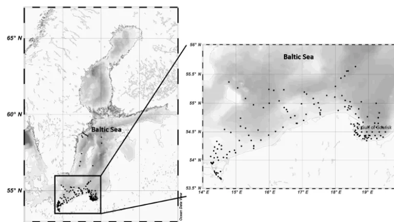
The empirical data used in this study were collected at more than 170 measuring stations in various parts of the southern and central Baltic Sea, though mainly in the Polish economic zone, from 2006 to 2014 (Fig. 1). These data were acquired principally during 42 short research cruises on board R/V
Oceaniaat different times of the year, but mostly from March to May and from September to October (about 80 % of the data analysed in this paper are from these periods). The prac-tice during each cruise was to select measuring stations that were maximally diverse with respect to their optical prop-erties, i.e. in the vicinity of river mouths and estuaries (the rivers Vistula, Oder, Reda, Łeba and ´Swina; the Szczecin Lagoon), bays and offshore waters (Gulf of Gda´nsk, Puck Bay and Pomeranian Bay), and open southern Baltic waters. During three cruises (in May of 2010, 2012 and 2014), mea-surements were also made in the open waters of the central Baltic. However, because of weather- and sea-state-related limitations, only 32 % of the data are from open-water
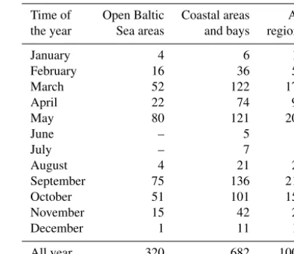
re-Table 1.Numbers of seawater samples analysed, divided into the months and areas of their acquisition.
Time of Open Baltic Coastal areas All the year Sea areas and bays regions
January 4 6 10
February 16 36 52
March 52 122 174
April 22 74 96
May 80 121 201
June – 5 5
July – 7 7
August 4 21 25
September 75 136 211 October 51 101 152 November 15 42 27
December 1 11 12
All year 320 682 1002
gions (Table 1). In addition to the cruise measurements, data were gathered throughout the year by sampling the seawater at the end of the ca. 400 m long pier in Sopot, on the Gulf of Gda´nsk coast (< 7 % of the overall number of data analysed). During the research cruises, a diversity of physical and op-tical parameters of seawater were measured in situ at each sampling station, and discrete seawater samples were col-lected for further laboratory analysis of certain optical prop-erties (spectra of coefficients of light absorption by phy-toplankton) and biogeochemical properties (concentrations of chlorophylla and other phytoplankton pigments). These samples were collected with a Niskin bottle (height ca. 0.9 m, capacity 25 L) immersed just below the surface; in shallow estuarine areas and river mouths (sampled from a pontoon) or off the end of the Sopot pier, they were obtained with a bucket. Immediately after collection, all samples were passed through glass fibre filters (Whatman, GF/F, 25 mm, nominal retention of particles with sizes down to 0.7 µm) at a pres-sure not exceeding 0.4 atm. The volumes filtered were cho-sen on a case-by-case basis; between 2 and 1150 mL of sea-water were filtered for later absorption measurements, and generally between 150 and 1000 mL were filtered for phyto-plankton pigment concentration analysis. All sample filters were immersed in a Dewar flask containing liquid nitrogen (at about−196◦C) and then kept frozen (at about −80◦C) for further analysis in the laboratory on land.
RSA-1526 J. Meler et al.: Parameterization of phytoplankton absorption in the Baltic Sea
Figure 1.Locations of all the sampling stations in the Baltic Sea; enlarged view of the study area.
UC-40). For the reference measurements we used clean fil-ters rinsed with particle-free seawater. The methodology of combined light-transmission and light-reflection measure-ments (known as the T–R method) was that described by Tassan and Ferrari (1995, 2002). From the pooled results of these measurements (several scans in different configu-rations), we calculated the optical density ODs(λ)
represent-ing each filtered sample. As opposed to standard spectropho-tometric analyses performed in transmission mode only, at least in theory, the results of T–R method should not need to be corrected for the so-called “scattering error”. But in order to calculate absorption coefficients of particles in so-lution, an additional correction has to be made to compen-sate for the elongation of the optical path of the light owing to the multiple scattering occurring in the filtered material. This is done by applying the dimensionless path length am-plification, theβ factor, which converts the measured opti-cal density of particles collected on the filter (ODs(λ))into
the optical density characterizing these particles in solution (ODsus(λ))(Mitchell, 1990). In our analyses we used the new
β-factor formula proposed by Stramski et al. (2015) for the T–R method:
ODsus(λ)=0.719ODs(λ)1.2287. (1)
The coefficient of light absorption by all suspended parti-cles was then calculated using the formula
ap(λ)= [ln(10)·ODsus(λ)]/ l, (2)
wherel(m) is the hypothetical optical path in solution, de-termined as the ratio of the volume of filtered water to the effective area of the filter. The absorption by non-algal parti-clesaNAP(λ)was determined in an analogous way, after the
phytoplankton pigments had been bleached for 2–3 min with a 2 % solution of calcium hypochlorite Ca(ClO)2 (Koblentz-Mishke et al., 1995; Wo´zniak et al., 1999); thereafter, the sample filter was rinsed with a small volume of particle-free seawater to remove any bleach residue, as this could addi-tionally absorb light at short wavelengths. Finally the sought-after coefficientaphwas calculated as the difference between
apandaNAP.
be-tween 740 and 750 nm was subtracted from the values ofaph across the entire spectrum. Generally different factors may have influenced the final uncertainty of our absorption mea-surements. Among them is the instrument noise present in each individual spectrophotometric scan (in each configura-tion) and also the possible uncertainty in path length ampli-fication factor, volume filtered and filter area used in subse-quent calculations, as well as uncertainty coming from sub-sampling from larger volumes of water. As a strict estimation of all these inaccuracies would be very complicated (due to the mathematical complexity of the algorithm used according to Tassan and Ferrari, 1995, 2002), here we limit ourselves only to estimating some of these inaccuracies. The mean in-accuracy caused by instrument noise occurring in separate measurements of light absorption by particles before and af-ter bleaching we estimated to be 1aph=5.68×10⁻³m−1 (±9.13×10⁻³m−1, standard deviation (SD)). We assumed that the uncertainty of aph (1aph) can be calculated as a square root of a sum of squares of uncertainties 1ap and
1aNAP. The latter were estimated as 95 % prediction inter-vals (=1.96 SD) for ap andaNAP values between 740 and 750 nm, where it is assumed that the absorption signal should be flat. Dividing the mean value of 1aph by correspond-ing measured values of aph(440) oraph(675) gave percent-age error distributions with mean values of 2.3 % and 5.9 %, respectively (with SD of 2.3 % and 7.6 %, respectively). In the collected dataset, due to logistic limitations, generally no measurements were made on multiple samples. However, in the separate tests we estimated the average uncertainty ofaph measurements due to subsampling to be 9.1 % (±1.5 %, SD). High performance liquid chromatography (HPLC) was used to determine phytoplankton pigment concentrations; the methodology is described in detail in Meler et al. (2017b), Sto´n and Kosakowska (2002), and Sto´n-Egiert and Kosakowska (2005). In this work we refer mainly to the total chlorophyllaconcentration (Tchla) (defined as the sum of chlorophylla, allomer and epimer, chlorophyllidea, and phaeophytina) and to the sum of the concentrations of all accessory pigments 6Ci, i.e. the sum of chlorophyllsb
(Tchlb), chlorophyllsc(Tchlc), photosynthetic carotenoids (PSC) and photoprotective carotenoids (PPC). The precision of HPLC measurements was estimated as equal to 2.9 % (±1.5 %, SD) and an error related to subsampling as 9.7 % (±6.4 %, SD) (Sto´n-Egiert et al., 2010).
The data were analysed statistically in order to character-ize their variability and to find approximate empirical rela-tionships between them. The variability of the target optical and biogeochemical quantities ranged over almost 3 orders of magnitude. Therefore, to assess the uncertainty of our empir-ical parameterizations, we applied standard arithmetic statis-tics of relative error and also separate statisstatis-tics of logarithmi-cally transformed data (so-called logarithmic statistics). The exact formulas are given as a footnote to Table 3 later in the paper.
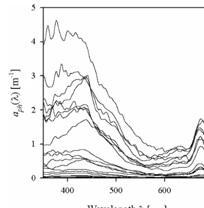
Figure 2.Examples of the spectra of the light absorption coefficient
aph(λ)representing the variability range of the data analysed in the
present paper.
3 Results and discussion
3.1 General characteristics of the data
Figure 2 exemplifies selected spectra ofaphthat we recorded in the Baltic Sea. Even though they were smoothed using the previously described raw data procedure, some still contain artefacts related to the noise occurring in our measurement system. These artefacts are particularly visible in the 350– 400 nm range, where the accuracy of measurements is lim-ited owing to the strong light attenuation by the glass fibre from which the filters are made, and also in the 550–650 nm range, where the absorption signal is small compared to other bands. In spite of these imperfections, 80 % of these spec-tra exhibit the expected characteristic absorption maxima in both the blue (ca. 440 nm) and red (ca. 675 nm) bands. Some of the spectra in our set, however, do not show a signifi-cant increase in light absorption with increasing wavelength in the 350–440 nm range: in 20 % of the spectra recorded
aph(400)/aph(440)is > 0.95 (in some cases as high as 1.42), mainly for samples from near the mouth of the River Vis-tula, in the Szczecin Lagoon and off the Sopot pier. The first part of Table 2 lists basic statistical information characteriz-ing the ranges of variation in the light absorption coefficient at selected light wavelengths. In fact, the variability ofaph(λ) over the entire spectral range examined, calculated for indi-vidual light wavelengths, was almost 3 orders of magnitude. For blue light, for example,aph(440) varied from 0.014 to 3.85 m−1, whereas for the local absorption maximum in the red band,aph(675) varied from 0.006 to 1.74 m−1.
1528 J. Meler et al.: Parameterization of phytoplankton absorption in the Baltic Sea
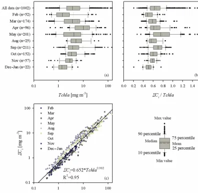
Figure 3. (a)Box plot presenting the range of variation in chlorophylla concentration (Tchla) for all the data analysed and for each sampling month;(b)as(a)but showing the ratio of the sum of accessory pigments to the chlorophyllaconcentration (6Ci/Tchla);(c)graph
illustrating the relationship between6Ci and Tchla– the solid line represents a simple functional approximation of the relationship (the
equation is given in the panel).
photosynthetic pigment chlorophyll a(Tchl a) and also the concentrations of different groups of accessory pigments, i.e. chlorophylls b and c, and other photosynthetic and photo-protective pigments (Tchl b, Tchlc, PSC and PPC). In ad-dition, the table lists the total concentration of all accessory pigments (6Ci) and the6Ci/Tchla ratio. Figure 3
illus-trates the variabilities of Tchlaand6Ci as well as their
ra-tio for all the pooled data, broken down into individual sam-pling periods (months). This shows that with respect to all the data analysed, the ranges of variability of both Tchl a
and6Ci are, like the absorption coefficient, almost 3 orders
of magnitude (0.41–141.8 and 0.15–72.1 mg m−3, respec-tively). The average Tchlafor all the data was 7.69 mg m−3. In the spring and summer months when we were able to make measurements at sea, mean values of Tchla were above av-erage, while in autumn and winter they were lower. In
gen-eral, a similar trend of average changes in individual months emerges from an analysis of the sum of accessory pigment concentrations6Ci. Taking into account all the data from
different periods of the year, we can say that measured val-ues of6Cicorrelate fairly well with Tchla(the approximate
equation and the coefficient of determinationR2 are given in Fig. 3c). Nevertheless, if we look at the6Ci/Tchla
ra-tio, we see that its average values also changed significantly during the year (Fig. 3b). The average 6Ci/Tchla for all
the data was 0.66, but the full range of variability that we recorded was from 0.21 to 1.5. For the months of April, May and September, the average6Ci/Tchlawas higher than or
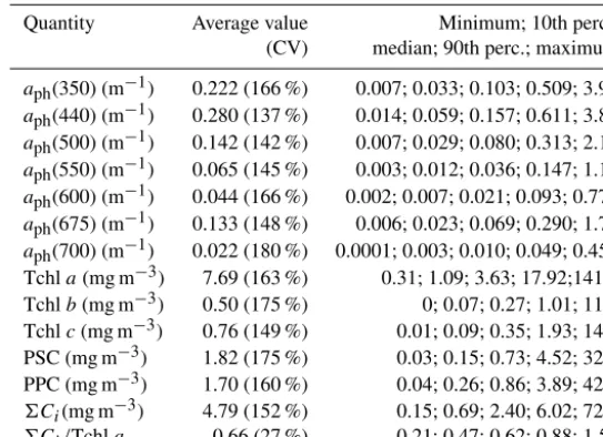
Table 2.Variability ranges of selected optical and biochemical quantities characterizing phytoplankton in samples from the Baltic Sea.
Quantity Average value Minimum; 10th perc.; (CV) median; 90th perc.; maximum
aph(350) (m−1) 0.222 (166 %) 0.007; 0.033; 0.103; 0.509; 3.91 aph(440) (m−1) 0.280 (137 %) 0.014; 0.059; 0.157; 0.611; 3.85 aph(500) (m−1) 0.142 (142 %) 0.007; 0.029; 0.080; 0.313; 2.17 aph(550) (m−1) 0.065 (145 %) 0.003; 0.012; 0.036; 0.147; 1.17 aph(600) (m−1) 0.044 (166 %) 0.002; 0.007; 0.021; 0.093; 0.772 aph(675) (m−1) 0.133 (148 %) 0.006; 0.023; 0.069; 0.290; 1.74 aph(700) (m−1) 0.022 (180 %) 0.0001; 0.003; 0.010; 0.049; 0.459
Tchla(mg m−3) 7.69 (163 %) 0.31; 1.09; 3.63; 17.92;141.8 Tchlb(mg m−3) 0.50 (175 %) 0; 0.07; 0.27; 1.01; 11.7 Tchlc(mg m−3) 0.76 (149 %) 0.01; 0.09; 0.35; 1.93; 14.8 PSC (mg m−3) 1.82 (175 %) 0.03; 0.15; 0.73; 4.52; 32.1 PPC (mg m−3) 1.70 (160 %) 0.04; 0.26; 0.86; 3.89; 42.8
6Ci(mg m−3) 4.79 (152 %) 0.15; 0.69; 2.40; 6.02; 72.1 6Ci/Tchla 0.66 (27 %) 0.21; 0.47; 0.62; 0.88; 1.50
solely the chlorophylla concentration as a simplified mea-sure to describe the overall pigment population and to which measure the light absorption of pigments is customarily pa-rameterized.
3.2 Approximate description of the light absorption coefficient by phytoplankton
3.2.1 General and monthly variants of one-component parameterizations
We carried out statistical analyses of our measurement data in order to define classic forms of the approximate functional relations between the light absorption coefficientaph(λ)and the concentration Tchl a. Like Bricaud et al. (1995, 1998), we approximated these relations using power functions. With linear regression applied to the logarithms of the input data for each light wavelength (regression between log(aph(λ)) and log(Tchla)), the coefficientsAandEof the following approximated parameterization could be calculated:
aph(λ)=A(λ)·TchlaE(λ). (3a)
Note that coefficientA(λ)determined in this way reflects the numerical value of the light absorption coefficientaph(λ)that the approximated relationship assigns to the case when the Tchlais exactly 1 mg m−3. The coefficientE(λ)of Eq. (3a) is a dimensionless quantity, which is the exponent of the power to which the chlorophylla concentration is raised. If its value is < 1, there is a statistical tendency for the phy-toplankton absorption efficiency to decrease per unit mass of chlorophyllawith increasing absolute chlorophylla concen-tration. A value ofE=1 would mean a stableaphto Tchla ratio, while a value of E> 1 would imply a statistical ten-dency foraph/Tchla to increase with increasing Tchla. By performing linear regression of the logarithms of the input
data, we were also able to calculate the determination co-efficients R2 for the approximated parameterization at the individual wavelengths of light. The parameterization coef-ficientsAandEgiven by Eq. (3a) can be easily used to de-termine the specific coefficient of light absorption by phyto-planktonaph∗(λ)(m2mg−1) (defined as values ofaph(λ) nor-malized with respect to Tchla):
aph∗ (λ)=A (λ)·TchlaE(λ)−1. (3b)
alter-1530 J. Meler et al.: Parameterization of phytoplankton absorption in the Baltic Sea
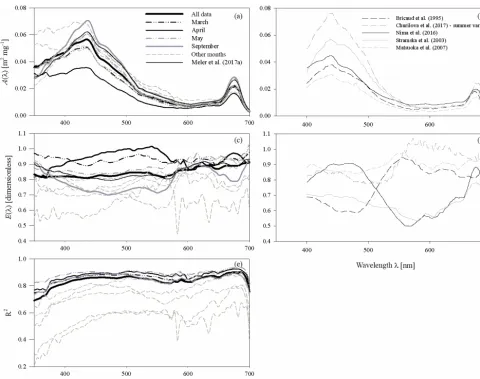
Figure 4. (a, c)Spectral plots of coefficientsAandEof the parameterizations described by Eq. (3a), and(e)the corresponding values of coefficientR2, determined for all the data analysed and for each sampling month. The coefficients of the preliminary parameterization given in Meler et al. (2017a) are also plotted;(b, d)examples of coefficientsAandEgiven by various authors (the legend is given inb).
native parameterizations over the entire spectral range. In the general variant, Echanges only slightly, between 0.81 and 0.91. On the other hand, the values of E for the parame-terizations derived for individual months are spectrally more differentiated, with more pronounced local maxima and min-ima. The deviations from the general case of the parameter-izations are the largest for March and April (upward) and for December–January (downward). The determination co-efficients R2, which may initially characterize the accuracy of the absorption coefficient parameterization using Eq. (3a), are relatively high in the case of the general variant of param-eterization, i.e. no less than 0.8, over almost the entire visible light range. Lower values ofR2are found only at the edges of the spectral range examined, where either the accuracy of measurements is expected to be lower (short wavelengths) or the values of the absorption coefficient are close to zero (long wavelengths). In the case of the monthly parameterizations,
only the formulas obtained for months with relatively large amounts of data take equally high values ofR2(i.e. March, April, May and September). For the other months, values of
R2are < 0.8, at least in significant parts of the spectral range examined.
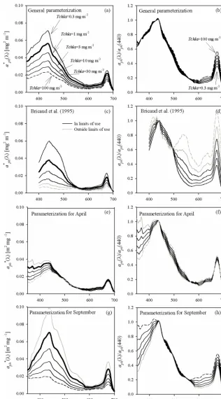
Figure 5.Example spectra of the specific coefficients of light absorption by phytoplanktonaph∗(λ)(left-hand column) and spectra ofaph
normalized to its own value in the 440 nm band (right-hand column) for some values of Tchlabetween 0.3 and 100 mg m−3:(a, b)estimated using the general variant of the parameterization obtained in this paper;(c, d)estimated on the basis of the parameterization by Bricaud et al. (1995) (the grey lines incanddrepresent chlorophyllaconcentrations Tchlathat go beyond the range for which the Bricaud et al. parameterization was originally developed);(e, f)estimated using the variant of parameterization obtained in this paper for April data only;
1532 J. Meler et al.: Parameterization of phytoplankton absorption in the Baltic Sea
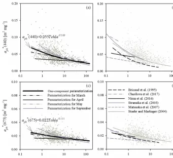
Figure 6. (a) Relationship between coefficient aph∗(440) and the chlorophyll aconcentration Tchl a and its functional approximations determined in this study for all the data analysed and for selected sampling months (the legend is given inc; the equation given in the panel represents approximations of all the data available; for coefficients obtained for particular months, see Table A2 in Appendix A);(c)as in
(a)but fora∗ph(675);(b, d)plots similar to(a, c)but presenting examples of functional approximations determined by various authors (the legend is given ind). The grey dots in each panel represent individual data points from our database.
visualize the “evolution” of the spectral shape of the pre-dicted spectra of aph, another family of curves is plotted. The spectra of aph, normalized with respect to 440 nm, are plotted in Fig. 5b and f for values of Tchla from the same range. To provide some background, Fig. 5c and d show two analogous diagrams obtained using the “classic” param-eterization developed by Bricaud et al. (1995) (although it should be mentioned that the two highest Tchlavalues – 30 and 100 mg m−3– generally lie beyond the range for which Bricaud et al. (1995) originally developed their parameteri-zation). Both parameterizations, our new one and the clas-sic one according to Bricaud et al. (1995), clearly predict drops inaph∗(λ)with increasing Tchla. But where changes in spectral shapes are concerned, our general parameterization predicts significant changes only in the 600–680 nm spec-tral range, whereas according to Bricaud et al. (1995) the variations should occur over a much broader spectral range (Fig. 5b and d). Both parameterizations qualitatively predict the well-known phenomenon of absorption spectra “flatten-ing” with increasing Tchla (e.g. Morel and Bricaud, 1981), but these predictions are quantitatively different. As a
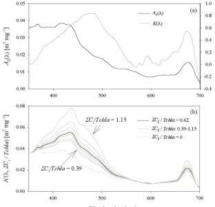
Figure 7. (a)Spectral plots of coefficientsA0andKof the two-component parameterization described by Eq. (4);(b)examples of curves
representing coefficentA0(λ,6Ci/Tchla), defined by Eq. (5), for the following values of6Ci/Tchla: the average value of 0.62; selected
values between 0.39 and 1.15 (representing the range from the 10th percentile for the December–January period to the 90th percentile for May); the hypothetical value of 0.
ofaph∗(λ)curves plotted for April (Fig. 5e) shows generally much lower values in the blue light maximum and less steep slopes around this maximum than the corresponding curves for September (Fig. 5g). Also, the variability in the normal-ized shapes of coefficientaphis greater and more complex for these two particular months (Fig. 5f to h) than was the case with the general parameterization (Fig. 5b). The colour index changes only by a factor of 1.16 (a drop from 2.2 to 1.9) for April, while for September the corresponding change is by a factor of 1.49 (a drop from 2.7 to 1.8). There are, more-over, differences in the evolution of slopes in the short-wave part of the spectrum between these two months that were not manifested by the general version of our parameterization.
Distinct differences between different months can also be visualized by plotting the mass-specific absorption coeffi-cients a∗ph at selected bands against chlorophyll a concen-trations. Figure 6a and c illustrate such plots for 440 and 675 nm bands. Evident differences in the slopes of approx-imate curves for the selected four months can be seen. Al-though for May and March we obtain slopes of thea∗ph vs. Tchlarelationships relatively close to those obtained for the whole dataset, quite different values are obtained for April and September.
3.2.2 Two-component parameterization
As already indicated in Sect. 3.1, there is a noticeable varia-tion in the proporvaria-tion between Tchlaand the concentrations of other phytoplankton pigments in particular months of the year within our dataset (Fig. 3). This variability initially indi-cated the limitations that may crop up when the chlorophylla
concentration is used as the only variable for parameterizing the spectra of aph(λ). Such limitations became clear when we recorded the differences between the parameterizations matched to the data from selected months. As a step towards improving the accuracy ofaph parameterization, while re-taining the relative simplicity of the mathematical formalism used, we decided to search for one additional variable. Dif-ferent candidates for this variable were tested: various ratios between concentrations of different groups of accessory pig-ment concentrations (Tchlb, Tchlc, PSC, PPC, their partial sums and the sum6Ci)and Tchla. As a result of these tests
we found that the best for this particular purpose was the ra-tio of all accessory pigments to chlorophylla(6Ci/Tchla).
1534 J. Meler et al.: Parameterization of phytoplankton absorption in the Baltic Sea
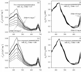
Figure 8.Example spectra of the specific coefficient of light absorption by phytoplanktonaph∗ (a, c)and spectra of coefficientaphnormalized
to its value in the 440 nm band(b, d), for some values of Tchlabetween 0.3 and 100 mg m−3, estimated by the two-component parameter-ization Eq. (4), and for two different assumed constant values of the pigment concentration ratio6Ci/Tchla: 0.47 (representing the 10th
percentile for all data) and 0.88 (representing the 90th percentile for all data).
was derived are given in Appendix B):
aph(λ)=A0(λ)·eK(λ)·
P
Ci
Tchla ·TchlaE(λ). (4)
The numerical coefficients of the new parameterization, i.e.
A0(λ)(m2mg−1) andK(λ)(no units), are summarized in Ta-ble A3 in Appendix A (with a spectral resolution of 2 nm). Note that coefficient E(λ)(no units) takes the same values as those in the general variant of the one-component param-eterization. Note, too, that the product of the new coefficient
A0(λ)and the exponential function appearing in Eq. (4) al-lows one, with the adopted value of the ratio 6Ci/Tchla,
to calculate the value corresponding to coefficientA(λ)from the parameterization given by Eq. (3a). We define this prod-uct as
A0
λ,
P
Ci
Tchla
=A0(λ)·eK(λ)·
P
Ci
Tchla. (5)
Spectral values of the new coefficients of Eq. (4) (coefficients
A0(λ)andK(λ))are shown in Fig. 7a, and Fig. 7b illustrates the family ofA0(λ,6Ci/Tchla) curves plotted for some
val-ues of6Ci/Tchlain our database.
As in the case of single-variable parameterizations, exam-ple families of aph∗ curves are now presented for the new two-component parameterization (Fig. 8) for two values of
6Ci/Tchla, i.e. 0.47 and 0.88, corresponding to the 10th
and 90th percentiles from the observed distribution of that ratio. There are conspicuous differences in this respect be-tween both the values and the shapes of the aph∗ spectra. As expected, the new two-component parameterization gen-erally predicts lower values of aph∗ (λ) for lower values of
6Ci/Tchla than for higher ones. If we assume a low
pro-portion of accessory pigments, i.e. for 6Ci/Tchla=0.47
vari-Figure 9.Comparison of the main characteristics of the estimation error logarithmic statistics calculated for various parameterizations of phytoplankton absorption coefficients:(a)the mean logarithmic errors of estimationhεig and(b)the standard error factorx. Dif-ferent curves in these panels represent the two-component parame-terization from this study, the preliminary parameparame-terization accord-ing to Meler et al. (2017a) and selected examples of parameteriza-tions gleaned from the literature (according to Bricaud et al., 1995; Churilova et al., 2017; Nima et al., 2016; Matsuoka et al., 2007; Stramska, 2003) (the legend is given in panelb). All these parame-terizations were applied to our entire dataset.
ability of parameterized light absorption spectra. But it also seems likely that even with the new two-component param-eterization, it will not be possible to explain all the differ-ences manifested by the monthly one-component parame-terizations. This intuitive expectation can be quantitatively checked by analysing in detail the estimation errors calcu-lated for different variants of the parameterizations.
3.3 Estimation errors of the different variants of parameterizations
We performed an extensive analysis of the errors arising out of the different variants of the proposed approximation for-mulas (analysis of estimation errors). Different cases were considered: the formulas were tested on the whole dataset as well as on data from particular months only. In our analy-ses we used both the arithmetic statistics of relative errors and also so-called logarithmic statistics, as these are gener-ally appropriate when the variation in tested/estimated
quan-tities spans several orders of magnitude. Below we present the most important results of these analyses.
1536 J. Meler et al.: Parameterization of phytoplankton absorption in the Baltic Sea
Table 3.Statistics of estimation errors∗of coefficientaph(λ)in selected spectral bands when the different variants of the parameterization
derived in this study were applied to the entire dataset (n=1002). The calculated values are given for three scenarios: when the general variant of the one-component parameterization was used; when variants specific to individual months were chosen (the first alternative value is given in parentheses); and when the two-component parameterization was used (the second alternative value is given in parentheses).
λ(nm) Arithmetic statistics of relative error Logarithmic statistics
systematic error statistical error systematic error standard error factor statistical error
hεi(%) σε(%) hεig(%) x σ+(%) σ−(%)
350 17.9 (16.0; 18.0) 68 (65; 68) 0 (−0.0;−0.1) 1.81 (1.75; 1.82) 81 (75; 82) −45 (−43;−45) 400 8.5 (7.7; 8.1) 45 (42; 43) 0 (−0.0;−01) 1.51 (1.48; 1.51) 51 (48; 51) −34 (−33;−34) 440 6.3 (5.2; 5.4) 39 (34; 35) 0 (−0.0;−0.1) 1.42 (1.38; 1.40) 42 (38; 40) −30 (−28;−28) 500 6.1 (5.2; 5.2) 37 (34; 34) 0 (−0.0;−0.2) 1.42 (1.38; 1.39) 42 (38; 40) −29 (−28;−28) 550 7.6 (6.7; 7.6) 42 (39; 43) 0 (−0.1;−0.1) 1.47 (1.44; 1.48) 48 (44; 48) −32 (−31;−33) 600 8.8 (8.1; 8.8) 47 (46; 48) 0 (−0.2;−0.1) 1.52 (1.49; 1.52) 52 (49; 52) −34 (−33;−34) 675 5.0 (4.2; 4.4) 34 (31; 32) 0 (−0.0;−0.2) 1.37 (1.34; 1.35) 37 (34; 36) −27 (−25;−26) 690 5.8 (5.4; 5.8) 37 (37; 38) 0 (−0.1;−0.2) 1.40 (1.39; 1.41) 40 (39; 41) −29 (−28;−29) 700 23.8 (21.8; 24.5) 199 (193; 194) −0.9 (−0.2; 0.8) 1.69 (1.70; 1.74) 69 (70; 74) −41 (−41;−42)
∗Arithmetic statistics of the relative error:
mean of the relative error (representing the systematic error according to arithmetic statistics):hεi =N−1
N
P
i=1
εi, whereε=(Pi
−Oi )
Oi ,Oirepresents
observed/measured values andPirepresents predicted/estimated values;
standard deviation of the relative error (representing the statistical error according to arithmetic statistics):σε=
v u u t1
N N
P
i=1 εi− hεi2
! .
Logarithmic statistics:
the mean logarithmic error (representing the systematic error according to logarithmic statistics):hεig=10
log
Pi Oi
−1, whereDlogPi
Oi
E
is the mean of
logPi
Oi
;
the standard error factor (the quantity which allows the range of statistical errors to be calculated according to logarithmic statistics):x=10σlog, whereσ logis the
standard deviation of the set logPi
Oi
;
statistical logarithmic errors (representing the range of statistical errors according to logarithmic statistics):σ−=1x−1,σ+=x−1.
been observed (Fig. 7b). However, comparison of the esti-mation errors associated with the two-component parame-terization with the scenario of using monthly variants of the one-component parameterization slightly favours the latter.
The above estimation errors were calculated over the en-tire available dataset. Therefore, these results do not address the question of how much more accurate the results might be if different variants of parameterization were tested on data from just one particular month. Table 4 gathers some results which address the latter question. It lists results ob-tained for data subsets limited to four separate months and to light wavelengths representing only selected bands where the phytoplankton absorption is relatively high. Addition-ally, for brevity, only certain characteristics of the logarith-mic statistics are presented. We generally found that using the monthly parameterization instead of a general variant for individual months often reduces the level of statistical er-ror according to both arithmetic and logarithmic statistics by only a small amount, although it may have a significant im-pact by strongly reducing the systematic error. Applying the general variant of the parameterization to particular months may overestimate or underestimate the values of coefficients
aph by a few percent to as much as 30 % and more in
Table 4. Selected characteristics of the estimation error logarithmic statistics calculated according to different parameterizations and for particular months: March, April, May and September (the numbers of data considered were 174, 96, 201 and 211, respectively).
Variant of One component general One component month specific Two component parameterization
Month λ systematic standard systematic standard systematic standard (nm) error error factor error error factor error error factor
hεig(%) x hεig(%) x hεig(%) x
March 400 −7.4 1.56 0 1.54 −9.8 1.54 440 1.7 1.44 0 1.42 −2.6 1.41 500 0.8 1.45 0 1.42 −3.3 1.43 675 −1.5 1.41 0 1.41 −4.8 1.39
April 400 24.9 1.46 0 1.44 25.3 1.45
440 17.3 1.42 0 1.39 17.9 1.39 500 13.4 1.43 0 1.38 13.9 1.38 675 11.8 1.33 0 1.31 12.2 1.32 May 400 −5.7 1.47 0 1.46 −0.6 1.43 440 −11 1.40 0 1.39 −2.6 1.34 500 −9.8 1.39 0 1.39 −1.7 1.34 675 −4.9 1.45 0 1.35 2.2 1.34 September 400 −1.7 1.41 0 1.41 −0.5 1.42 440 −7.5 1.33 0 1.31 −5.6 1.33 500 −4.6 1.41 0 1.31 −2.7 1.33 675 −8.5 1.35 0 1.32 −7.0 1.34
3.4 Comparison with selected examples of parameterizations from the literature
So far, when discussing our own results, we have referred only to the classic version of the parameterization given by Bricaud et al. (1995). Now we shall briefly compare our re-sults with other examples of parameterizations from the liter-ature. In Fig. 5d and e we have plotted the coefficients of the parameterization by Bricaud et al. (1995), as well as coef-ficients of four other variants obtained for different marine environments by different authors: Stramska et al. (2003), Matsuoka et al. (2007), Nima et al. (2016) and Churilova et al. (2017). These examples were chosen from among the many known in the literature, in order to illustrate the pos-sible variability occurring between coefficients of different parameterizations that were originally matched to different datasets. In the case of coefficientsA, all the spectral shapes presented in Fig. 5d generally reflect the characteristic ab-sorption maxima in the blue and red spectral ranges. Quanti-tatively, however, there are significant differences between these examples, the largest being in the wavelength range from about 400 to 480 nm. Interestingly, such a range of co-efficient Avariability resembles the one we obtained with our own Baltic data when we developed separate variants of the one-component parameterization for individual months (Fig. 5a). With regard to the values of coefficients E, the literature examples presented in Fig. 5e differ significantly from each other and all exhibit a distinct variation in values
across the spectrum. According to these literature sources, coefficientsE can take values from less than 0.5 to even more than 1 in different spectral ranges. In our analyses we also found spectral variations in E values but only for pa-rameterization variants that were matched to the data from separate months; on pooling all our data, we found that the resulting spectral shape of coefficientE was relatively flat (with values between 0.8 and 0.9 for the general parame-terization variant) (Fig. 5b). The fact that the various liter-ature parameterizations clearly differ in their coefficientsE
can be additionally illustrated by different slopes of curves plotted on graphs showing estimated dependences of specific absorption coefficientsaph*(440) andaph*(675) as functions of Tchla (Fig. 6b and d). In addition to the examples men-tioned earlier, we also plotted curves according to Staehr and Markager (2004) as examples representing a wide range of Tchl a. Again, we would like to point out that the pattern of different slopes among literature examples resembles the differences we obtained from analysing the data for different months.
1538 J. Meler et al.: Parameterization of phytoplankton absorption in the Baltic Sea
our dataset. The systematic estimation errors ofaph(λ)in the classic parameterization according to Bricaud et al. (1995) range from−57 % to−21 % over almost the entire spectral range. Other examples show significant systematic errors at least in some portions of the light spectrum analysed (from almost−60 % to about+60 % at some cases). In Fig. 9a we also plotted systematic errors calculated now for our own, previous preliminary version of the Baltic Sea parameteriza-tion (Meler et al., 2017a). We now see that, apart from the UV range, values ofaphare generally overestimated by up to 20 % and more by this earlier version of the formula. With re-gard to the standard error factor, we can see that only some of the literature examples in the vicinity of phytoplankton light absorption peaks achieve similarly low values as represented by our new two-component parameterization. But since for the total estimation accuracy the contributions of both sys-tematic and statistical errors have to be taken into account, one can expect that overall, none of the literature examples can attain the accuracy that we achieved by matching our new parameterizations to our own dataset.
4 Final remarks
The empirical material for this work was acquired in a rel-atively small geographical area, mainly the southern Baltic Sea. However, because it was gathered in various parts of this basin, from coastal areas to open waters, and at differ-ent times of the year, the recorded light absorption coeffi-cients and concentrations of phytoplankton pigments have large ranges of variability, in both cases reaching almost 3 orders of magnitude. Based on such a dataset, it was possi-ble to derive a number of new variants of the parameteriza-tion of coefficient aph: they should be treated as simplified and practical relationships of a local character, tailored to the specifics of the target environment. The new empirical formulas include classic one-component parameterizations, where the only variable is the concentration of chlorophylla. Parameterizations of this type have been developed both as a general version, i.e. one matched to all the data collected in different periods of the year, and in the form of sepa-rate variants adjusted to the individual months of data collec-tion. Importantly, we found that the coefficients of monthly variants could differ from each other very significantly, thus indirectly reflecting the annual variation in the proportions between chlorophyll a and other photosynthetic or photo-protective pigments. The paper also presents a new, slightly more complex form of parameterization that uses one addi-tional variable: the ratio of the concentrations of accessory pigments to the concentration of chlorophylla.
With all the variants of this parameterization, spectra of coefficientaph can be estimated fairly simply and with few requirements as to input data. Such estimates can be made over a wide spectral range (from 350 to 700 nm) and with a high spectral resolution (1 nm). It should be borne in mind,
however, that the accuracy of such estimates is obviously limited. For example, the application of the general version of the one-component parameterization to all our data cov-ering different periods of the year understandably leads to practically zero systematic error of this estimate, although a significant statistical error remains. The latter may be charac-terized by standard error factors from 1.37 to 1.51 in the vast majority of the spectral ranges tested. However, since the real values ofaphvary in Baltic Sea conditions over almost 3 or-ders of magnitude, even an estimation accuracy such as this appears satisfactory. Our study has also shown that further improvement in the accuracy of the approximate description of aph spectra is possible, at least in some applications. In the case of datasets acquired at different times of the year, such an improvement can be achieved by using either “dy-namically selected” monthly variants of parameterizations, or, when pigment composition data are available, by using the new two-component parameterization. In the case of data limited to particular months, it is possible to prevent the oc-currence of significant systematic errors especially by using the appropriately selected monthly parameterization.
An important qualitative observation from our analyses is that the new variants of monthly parameterizations have a range of variability of coefficients similar to that between the different literature parameterizations established on the ba-sis of data from diverse aquatic environments. This particu-lar observation reminds us that all such parameterizations are always quite far-reaching simplifications of relationships oc-curring in nature. The variability of these relationships that we recorded throughout the year in the Baltic Sea seems to indicate that only the use of a much more elaborate mathe-matical apparatus, using a much larger number of variables describing the composition of pigments and other features of the phytoplankton population, could further and more radi-cally improve the accuracy of the spectral description of the light absorption coefficient (see, e.g., the multi-component models presented earlier in the papers by Wo´zniak et al., 1999, 2000a, b; Majchrowski et al., 2000; Ficek et al., 2004). In our opinion, however, the practical value of the simple pa-rameterizations presented in this work should be seen in the opportunities for applying them to the development of vari-ous methods and algorithms, whose specificity from the very beginning requires the use of simplifications.
Appendix A
1540 J. Meler et al.: Parameterization of phytoplankton absorption in the Baltic Sea
Table A1.Spectral coefficientsAandEof the one-component parameterization described by Eq. (3a) in its general variant (i.e. the variant obtained when all data, regardless of the month of acquisition, were taken into account) and the corresponding determination coefficientsR2.
λ(nm) A E R2 λ(nm) A E R2 λ(nm) A E R2
1 2 3 4 1 2 3 4 1 2 3 4
Table A2.Spectral coefficientsAandEof the one-component parameterization described by Eq. (3a) in its variants obtained in selected months and the corresponding determination coefficientsR2.
March April May September
λ(nm) A E R2 A E R2 A E R2 A E R2
1 2 3 4 2 3 4 2 3 4 2 3 4
1542 J. Meler et al.: Parameterization of phytoplankton absorption in the Baltic Sea
Table A3.Spectral coefficientsA0andKof the two-component parameterization described by Eq. (4). The other coefficientEis the same
as in the case of the one-component parameterization (see Table A1).
λ(nm) A0 K λ(nm) A0 K λ(nm) A0 K
1 2 3 1 2 3 1 2 3
Appendix B
In order to derive the two-component parameterization, the relationship described earlier by Eq. (3a) was treated as a first, intermediate stage in its construction (the examples are plotted at two wavelengths in Fig. B1a and b). To distinguish between them, the values calculated according to Eq. (3a) are now denoted aph(λ)cal, whereas the actually measured values of the absorption coefficient areaph(λ)m. In the next step, the relationship between the ratio aph(λ)cal/aph(λ)m and the ratio of the sum of accessory pigments to the con-centration of chlorophyll a6Ci/Tchla was analysed.
Fig-ure B1c and d illustrate the frequency distributions of the ra-tioaph(λ)cal/aph(λ)m, while Fig. B1e and f show the relation-ships between the ratiosaph(λ)m/aph(λ)caland6Ci/Tchla.
Despite the large dispersion of individual data points on the latter two panels, the general tendency for the logarithm of
aph(λ)m/aph(λ)calto decrease with increasing6Ci/Tchlais
evident. This tendency can be approximated by a linear func-tion, which effectively allows one to establish coefficients of an approximate exponential relationship between the two ra-tios investigated:
aph(λ)cal
aph(λ)m =f
PC
i
Tchla
=const1(λ)econst2(λ) P
Ci
Tchla. (B1)
Relationships of this form were determined over the entire spectral range (350–700 nm) with a step of 1 nm. Obviously, the determination coefficientsR2of the approximations are low, but this procedure generally permits additional informa-tion on the influence of pigment composiinforma-tion on the ultimate values of aph to be taken into account. Having the statisti-cal dependences described by first stage Eq. (3a) and sec-ond stage Eq. (B1) to hand, a new expression can be written that approximatesaph(λ)by treating it as a function of two variables at each light wavelength – chlorophylla concentra-tion (Tchla (mg m−3)) and the ratio of the sum of the con-centrations of the other accessory pigments to chlorophylla
(6Ci/Tchla):
aph(λ)=A0(λ)·eK(λ)·
P
Ci
Tchla ·TchlaE(λ). (B2)
The numerical coefficients of the newly obtained pa-rameterization, i.e. A0(λ) (m2mg−1) (where A0(λ)=
A(λ)/const1(λ)) and K(λ) (no units) (where K(λ)= −const2(λ)), are summarized in Table A3 in Appendix A. CoefficientE(λ)(no units) takes the same values as those in the general variant of the one-component parameterization.
Figure B1. (a, b) Relations between measured coefficients of absorption by phytoplankton (denoted by aph(λ)m) and
chloro-phyllaconcentrations for two light wavelengths (400 and 675 nm) and their functional approximations according to Eq. (3a) (the equations are given in the panels); (c, d) frequency distribu-tion histograms of the ratio of calculated and measured absorp-tion coefficients (aph(λ)cal/aph(λ)m); (e, f) relations between
the ratioaph(λ)cal/aph(λ)m and the pigment concentration ratio 6Ci/Tchlaand their functional approximations (the equations are
1544 J. Meler et al.: Parameterization of phytoplankton absorption in the Baltic Sea
Author contributions. JM and SBW directly participated in the planning and implementation of analyses presented in this study. JS-E participated in acquisition of empirical data. BW was the orig-inator of selected ideas explored in this work.
Competing interests. The authors declare that they have no conflict of interest.
Acknowledgements. The data used in this work were gathered with financial assistance from the “SatBałtyk” project funded by the European Union through the European Regional Development Fund (no. POIG.01.01.02-22-011/09, “The Satellite Monitoring of the Baltic Sea Environment”) and within the framework of the Statutory Research Project (no. I.1 and I.2) of the Institute of Oceanology Polish Academy of Sciences. The subsequent analyses of the data were carried out as part of project N N306 041136, financed by the Polish Ministry of Science and Higher Education in 2009-2014 (grants awarded to Bogdan Wo´zniak and Justyna Meler), and also the project funded by the National Science Centre, Poland, entitled “Advanced research into the relationships between optical, biogeochemical and physical properties of suspended particulate matter in the southern Baltic Sea” (contract no. 2016/21/B/ST10/02381) (awarded to Sławomir B. Wo´zniak) We thank Barbara Lednicka, Monika Zabłocka, Agnieszka Zdun and other colleagues from IOPAS for their help in collecting the empirical material.
Edited by: Oliver Zielinski
Reviewed by: two anonymous referees
References
Babin, M. and Stramski, D.: Light absorption by aquatic particles in the near-infrared spectral region, Limnol. Oceanogr., 47, 911– 915, 2002.
Babin, M., Stramski, D., Ferrari, G. M., Claustre, H., Bricaud, A., Obolensky, G., and Hoepffner, N.: Variations in the light ab-sorption coefficient of phytoplankton, nonalgal particles, and dis-solved organic matter in coastal waters around Europe, J. Geo-phys. Res., 108, 3211, https://doi.org/10.1029/2001JC000882, 2003.
Bidigare, R., Ondrusek, M. E., Morrow, J. H., and Kiefer, D. A.: “In vivo” absorption properties of algal pigments, Ocean. Opt., 10, 290–302, 1990.
Bricaud, A., Babin, M., Morel, A., and Claustre, H.: Variability in the chlorophyll-specific absorption coefficients of natural phyto-plankton: Analysis and parameterization, J. Geophys. Res., 100, 13321–13332, 1995.
Bricaud, A., Morel, A., Babin, M., Allali, K., and Claustre, H.: Vari-ations of light absorption by suspended particles with chlorophyll a concentration in oceanic (case 1) waters: analysis and impli-cations for bio-optical models, J. Geophys. Res., 103, 31033– 31044, 1998.
Bricaud, A., Claustre, H., Ras, J., and Oubelkheir, K.: Natural vari-ability of phytoplankton absorption in oceanic waters: influence
of the size structure of algal populations, J. Geophys. Res., 109, C11010, https://doi.org/10.1029/2004JC002419, 2004.
Churilova, T., Suslin, V., Krivenko, O., Efimova, T., Moiseeva, N., Mukhanov, V., and Smirnova, L.: Light absorption by phytoplankton in the upper mixed layer of the Black Sea: seasonality and parameterization, Front. Mar. Sci., 4, 90, https://doi.org/10.3389/fmars.2017.00090, 2017.
Dmitriev, E. V., Khomenko, G., Chami, M., Sokolov, A. A., Churilova, T., and Korotaev, G. K.: Parameterization of light ab-sorption by components of seawater in optically complex coastal waters of the Crimea Penisula (Black Sea), Appl. Opt., 48, 1249– 1261, 2009.
Ficek, D., Meler, J., Zapadka, T., Wo´zniak, B., and Dera, J.: Inherent optical properties and remote sensing reflectance of Pomeranian lakes (Poland), Oceanologia, 54, 611–630, 2012a.
Ficek, D., Meler, J., Zapadka, T., and Sto´n-Egiert, J.: Modelling the light absorption coefficients of phytoplankton in Pomera-nian lakes (Northern Poland), Fund. Appl. Hydrophys., 5, 54–63, 2012b.
Ficek, D., Kaczmarek, S., Sto´n-Egiert, J., Wo´zniak, B., Ma-jchrowski, R., and Dera, J.: Spectra of Light absorption by phyto-plankton pigments in the Baltic; conclusions to be drawn from a Gaussian analysis of empirical data, Oceanologia, 46, 533–555, 2004.
Kirk, J. T. O.: Light and Photosynthesis in Aquatic Ecosystems, Cambridge University Press, London-New York, 509, 1994. Koblentz-Mishke, O. I., Wo´zniak, B., Kaczmarek, S., and
Kono-valov, B. V.: The assimilation of light energy by marine phyto-plankton, Part 1, The light absorption capacity of the Baltic and Black Sea phytoplankton (methods; relation to chlorophyll con-centration), Oceanologia, 37, 145–169, 1995.
Kowalczuk, P.: Seasonal variability of yellow substance absorption in the surface layer of the Baltic Sea, J. Geophys. Res., 104, 30047–30058, 1999.
Majchrowski, R., Wo´zniak, B., Dera, J., Ficek, D., Kaczmarek, S., Ostrowska, M., and Koblentz-Mishke, O. I.: Model of the in vivo spectral absorption of algal pigments, Part 2, Practical applica-tions of the model, Oceanologia, 42, 191–202, 2000.
Mascarenhas, V. J. and Zielinski, O.: Parameterization of spectral particulate and phytoplankton absorption coeffi-cients in Sognefjord and Trondheimsfjord, two contrast-ing Norwegian Fjord ecossytems, Remote Sens., 10, 977, https://doi.org/10.3390/rs10060977, 2018.
Matsuoka, A., Hout, Y., Shimada, K., Saitoh, S., and Babin, M.: Bio-optical characteristics of the western Artic Ocean: implica-tions for ocean color algorithms, Can. J. Remote Sensing, 33, 503–518, 2007.
Meler, J., Kowalczuk, P., Ostrowska, M., Ficek, D., Zablocka, M., and Zdun, A.: Parameterization of the light absorption properties of chromophoric dissolved organic matter in the Baltic Sea and Pomeranian lakes, Ocean Sci., 12, 1013–1032, https://doi.org/10.5194/os-12-1013-2016, 2016a.
Meler, J., Ostrowska, M., and Sto´n-Egiert, J.: Seasonal and spatial variability of phytoplankton and non-algal absorption in the sur-face layer of the Baltic, Estuar. Coast. Shelf S., 180, 123–135, https://doi.org/10.1016/j.ecss.2016.06.012, 2016b.
re-mote sensing applications, Oceanologia, 59, 195–212, https://doi.org/10.1016/j.oceano.2017.03.010, 2017a.
Meler, J., Ostrowska, M., Sto´n-Egiert, J., and Zabłocka, M.: Sea-sonal and spatial variability of light absorption by suspended par-ticles in the southern Baltic: a mathematical description, J. Mar. Sys., 170, 68–87, https://doi.org/10.1016/j.jmarsys.2016.10.011, 2017b.
Mitchell, B. G.: Algorithm for determining the absorption coef-ficient of aquatic particulates using the quantitative filter tech-nique, Proc. SPIE., 1302, 137–148, 1990.
Mitchell, B. G., Kahru, M., Wieland, J., and Stramska, M.: Determi-nation of spectral absorption coefficients of particles, dissolved material and phytoplankton for discrete water samples, in: Ocean Optics Protocols For Satellite Ocean Color Sensor Validation, edited by: Fargion, G. S. and Mueller, J. L., Revision 3, Vol. 2, NASA Technical Memorandum 2002-210004/Rev 3-Vol 2, 15, 231–257, 2002.
Mobley, B. D.: Light and Water, Radiative Transfer in Natural Wa-ters, Acad. Press, San Diego, 592 pp., 1994.
Morel, A. and Bricaud, A.: Theoretical results concerning light absorption in a discrete medium, and application to specific absorption of phytoplankton, Deep-Sea-Res., 28, 1375–1393, https://doi.org/10.1016/0198-0149(81)90039-X, 1981.
Morel, A. and Bricaud, A.: Inherent optical properties of algal cells including picoplankton: theoretical and experimental results, in: Photosynthetic picoplankton, edited by: Platt, T. and Li, W. K. W., Can. Bull. Fish. Aquat. Sci., 214, 521–559, 1986.
Nima, C., Frette, Ø., Hamre, B., Erga, S., Chen, Y., Zhao, L., Sørensen, K., Norli, M., Stamnes, K., and Stamnes, J.: Absorp-tion properties of high-latitude Norwegian coastal water: The im-pact of CDOM and particulate matter, Estuar. Coast. Shelf S., 178, 158–167, https://doi.org/10.1016/j.ecss.2016.05.012, 2016. Paavel, B., Kangro, K., Arst, H., Reinart, A., Kutser, T., and No-ges, T.: Parameterization of chlorophyll-specific phytoplankton absorption coefficients for productive lake waters, J. Limnol., 75, 423–438, 2016.
Reinart, A., Paavel, B., Pierson, D., and Strömbeck, N.: Inherent and apparent optical properties of Lake Peipsi, Estonia, Boreal Environ. Res., 9, 429–445, 2004.
Staehr, P. A. and Markager, S.: Parameterization of the chlorophyll a-specific in vivo light absorption coefficient covering estuarine, coastal and oceanic waters, Int. J. Remote Sens., 25, 5117–5130, 2004.
Sto´n, J. and Kosakowska, A.: Phytoplankton pigments designation – an application of RP-HPLC in qualitative and quantitative anal-ysis, J. Appl. Phycol., 14, 205–210, 2002.
Sto´n-Egiert, J. and Kosakowska, A.: RP-HPLC determination of phytoplankton pigments comparison of calibration results for two columns, Mar. Biol., 147, 251–260, 2005.
Sto´n-Egiert, J., Łotocka, M., Ostrowska, M., and Kosakowska, A.: The influence of biotic factors on phytoplankton pigment compo-sition and resources in Baltic ecosystems: new analytical results, Oceanologia, 52, 101–125, 2010.
Stramska, M., Stramski, D., Hapter, R., Kaczmarek, S., and Sto´n, J.: Bio-optical relationships and ocean color algorithms for the north polar region of the Atlantic, J. Geophys. Res., 108, 3143, https://doi.org/10.1029/2001JC001195, 2003.
Stramski, D., Reynolds, R. I., Kaczmarek, S., Uitz, J., and Zheng, G.: Correction of pathlength amplification in the filter-pad
tech-nique for measurements of particulate absorption coefficient in the visible spectral region, Appl. Opt., 54, 6763–6782, 2015. Tassan, S. and Ferrari, G. M.: An Alternative Approach to
Absorp-tion Measurements of Aquatic Particles Retained on Filters, Lim-nol. Oceanogr., 40, 1358–1368, 1995.
Tassan, S. and Ferrari, G. M.: A sensitivity analysis of the “Transmittance-Reflectance” method for measuring light ab-sorption by aquatic particles, J. Plankton Res., 24, 757–774, https://doi.org/10.1093/plankt/24.8.757, 2002.
Thamm, R., Schernewski, G., Wasmond, N., and Neumann, T.: Spa-tial phytoplankton in the Baltic Sea, in: Baltic Sea typology, edited by: Schernewski, G. and Wielgat, M., Costline Reports, 4, 85–109, 2004.
Trees, C., Clark, D., Bidigare, R., Ondrusek, E., and Mueller, J.: Accessory pigments versus chlorophyll a concentrations within the euphotic zone: A ubiquitous relationship, Limnol. Oceanogr., 45, 1130–1143, 2000.
Wasmund, N. and Uhlig, S.: Phytoplankton in large river plumes in the Baltic Sea, ICES J. Mar. Sci., 56, 23–32, 2003.
Wasmund, N., Breuel, G., Edler, L., Kuosa, H., Olsonen, R., Schultz, H., Pys-Wolska, M., and Wrzołek, L.: Pelagic biology, in: Third Periodic Assessment of the State of Marine Environ-ment of the Baltic Sea, 199–93; Background docuEnviron-ment, Baltic Sea Environment Proceedings No. 64B, Helsinki Commission, 89–93, 1996.
Wasmund, N., Andrushaitis, A., Łysiak-Pastuszak, E., Müller-Karulis, B., Nausch, G., Neumann, T., Ojaveer, H., Olenina, I., Postel, L., and Witek, Z.: Trophic status of the south-eastern Baltic Sea: a comparison of coastal and open areas, Estuar. Coast. Shelf Sci., 53, 849–864, 2001.
Witek, B. and Pli´nski, M.: Occurrence of blue-green algae in the phytoplankton of the Gulf of Gda´nsk in the years 1994–1997, Oceanological Stud., 3, 77–82, 1998.
Wo´zniak, B. and Ostrowska, M.: Composition and resources of pho-tosynthetic pigments of the sea phytoplankton, Oceanologia, 29, 91–115, 1990a.
Wo´zniak, B. and Ostrowska, M.: Optical absorption properties of phytoplankton in various seas, Oceanologia, 29, 147–174, 1990b. Wo´zniak, B. and Dera, J.: Light Absorption in Sea Water, Springer,
New York, 2007.
Wo´zniak, B., Dera, J., Ficek, D., Majchrowski, R., Kaczmarek, S., Ostrowska, M., and Koblentz-Mishke, O. I.: Modelling the influ-ence of acclimation on the absorption properties of marine phy-toplankton, Oceanologia, 41, 187–210, 1999.
Wo´zniak, B., Dera, J., Ficek, D., Majchrowski, R., Kaczmarek, S., Ostrowska, M., and Koblentz-Mishke, O. I.: Model of the “in vivo” spectral absorption of algal pigments, Part 1, Mathematical apparatus, Oceanologia, 42, 177–190, 2000a.
Wo´zniak, B., Dera, J., Ficek, D., Majchrowski, R., Kaczmarek, S., Ostrowska, M., and Koblentz-Mishke, O. I.: Model of the “in vivo” spectral absorption of algal pigments, Part 2, Practical ap-plications of the model, Oceanologia, 42, 191–202, 2000b. Ylöstalo, P., Kallio, K., and Seppälä, J.: Absorption properties of