A High-Frequency Model of a Rectilinear Beam with a T-Shaped Cross Section

(1)

acoustics

Article

A High-Frequency Model of a Rectilinear Beam with a

T-Shaped Cross Section

Andrew J. Hull *, Daniel Perez and Donald L. Cox

Naval Undersea Warfare Center, Newport, RI 02841, USA

* Correspondence: [email protected]; Tel.:+1-401-832-5189

Received: 3 June 2019; Accepted: 26 August 2019; Published: 9 September 2019

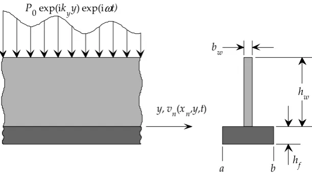
Abstract:This paper derives an analytical model of a straight beam with a T-shaped cross section for use in the high-frequency range, defined here as approximately 1 to 35 kHz. The web, the right part of the flange, and the left part of the flange of the T-beam are modeled independently with two-dimensional elasticity equations for the in-plane motion and Mindlin flexural plate equation for the out-of-plane motion. The differential equations are solved with unknown wave propagation coefficients multiplied by circular spatial domain functions. These algebraic equations are then solved to yield the wave propagation coefficients and thus produce a solution to the displacement field in all three directions. An example problem is formulated and compared with solutions from fully elastic finite element modeling, a previously derived analytical model, and Timoshenko beam theory. It is shown that the accurate frequency range of this new model is significantly higher than that of the analytical model and the Timoshenko beam model, and, in the frequency range up to 35 kHz, the results compare very favorably to those from finite element analysis.

Keywords: rectilinear beam; T section; beam vibrations; high-frequency response

1. Introduction

This paper is a direct extension of a previous effort [1,2] that modeled the dynamics of a straight T-beam. This model accurately captured the physics of the beam up to about 8 kilohertz (kHz) for the example problem studied. The previous beam model became inaccurate above 8 kHz because of the limitations of the out-of-plane (normal) component, which was a Love-Kirchhoff[3] plate formulation. The assumptions of the Love-Kirchhoff plate equations typically produce model results that are too stiff, especially as the frequency increases. In the new model derived here, the Love-Kirchhoff plate equations are replaced by Mindlin plate equations [4], whose theoretical basis includes shear deformation and rotary inertia terms, resulting in a higher-frequency range of analysis. This permits the new analytical model of a straight T-shaped beam to extend the frequency range of this system compared to previous modeling efforts. It is primarily intended for use in models that have reinforced plates that need improved accuracy at higher frequencies.

Beams are structural members and are designed to resist an external force either applied directly or applied to a body that they are supporting. They provide a concentrated or distributed stiffness in a mechanical system that has various design objectives. There is an extremely large body of analytical and experimental papers that model and analyze various types of beams. The first equation for the motion of a beam was developed by Bernoulli and Euler [5], and this equation is presented in almost every text on mechanical vibrations. This theory uses the assumption that all sections rotate orthogonally to the neutral axis of the beam. Timoshenko [6] revised this equation so that the rotation angle was a function of the shear effects and polar inertia of the beam. Beam theory has been made more accurate by the inclusion of higher-order displacement functions, usually in the axial direction. Bickford [7] used a third-order polynomial through the thickness of the beam to model the in-plane

(2)

Acoustics2019,1 727

displacement field. Karama et al. [8] used an exponential function to model the shear distribution in the beam. Other functional distributions [9] are possible and have also been similarly applied to plate theory. These higher-order models are lumped parameter models and do not have the ability to model higher-frequency wave motion in the normal direction of the beam.

Beam shapes have become more geometrically diverse and their cross sections have been modified from rectangular to L-, T-, I-, and H-shaped, channel-shaped, and hollow box designs. Park et al. [10] studied the longitudinal wave motion of finite coupled thin plates. Kessissoglou [11] added the flexural motion to the previous reference so that a full three-dimensional analysis of an L-shaped finite plate became possible. Du et al. [12] investigated the free vibration of coupled rectangular plates with general boundary conditions, using energy methods to derive the differential equations of motion. Chen et al. [13] analyzed vibrations in box-type plate structures. Wang [14] addressed the problem of finite coupled plates whose intersection contained a mass. T-shaped beams have been the subject of some investigations [15,16], generally applied to concrete or reinforced concrete structures where static analysis and ultimate strength are the major foci of the research. Langley and Heron [17] derived a method to calculate the wave transmission coefficients of plate and beam junctions. Keir et al. [18] investigated coupled rectangular plates, with an emphasis on the effect of active control of these systems. Mitrou et al. [19] researched wave transmission in two-dimensional structures using a mixed finite element and wave and finite element methods.

Beam-reinforced structures have been analyzed for many years. Fluid-loaded stiffened plates have been researched using flexural wave plate models by Mace [20,21] and Lin and Hayek [22], with a general emphasis on structural acoustic responses. The plate governing equations in a stiffened plate analysis has been extended to admit fully elastic wave propagation by Hull and Welch [23], and this allows much higher-frequency studies compared to previous flexural wave models. Models of these structures typically have an infinite length assumption as the energy propagates down the length of the structure and, due to the large spatial lengths and slight damping present, does not form a standing wave pattern. The model of the beam reinforcement has typically been an infinite length Bernoulli-Euler or Timoshenko model, which has very low to low frequency range limitations.

This paper develops an analytical model of a T-shaped beam for high-frequency range analysis. In this model, the web and flange of the T-beam are modeled independently with two-dimensional elasticity equations accounting for the in-plane motion and the Timoshenko plate equations accounting for the out-of-plane motion. The method presented here combines six in-plane components and six out-of-plane components into a single model that can predict the response of a T-beam to various external loads. The web and flange are joined by 12 equilibrium and constraint equations and the free and forced edges are modeled with 12 additional force and moment equations. Modeling the beam in this manner allows the web and flange equations of motion to incorporate coupled in-plane and out-of-plane plate responses, and these equations make the model much more accurate compared to previous shear deformation models [7,8]. For the specific example presented in this paper, the three-dimensional displacement fields are studied with respect to independent loads in the three primary axes of the Cartesian coordinate system. Comparisons are made to a previous analytical model, a Timoshenko beam model, and a finite element model. It is shown that, for the specific example presented here, the accurate frequency region of the normal displacement divided by normal pressure is increased from 1 kHz of the Timoshenko beam model, or 8 kHz of the previous analytical model, to 35 kHz for the new beam model. Beam mode shapes are also calculated.

2. Methods

(3)

Acoustics2019,1 728

the two-dimensional plane stress elastic equations for in-plane motions of the web and the flange, and Mindlin plate equations are used for the out-of-plane motion of the web and the flange. This model is an extension of a previous model wherein the classical plate equation was used to model the out-of-plane motions. The model makes the following assumptions: (1) the system has infinite spatial extent in they-direction, (2) the excitation is at a fixed frequency and fixed wavenumber in the y-direction, (3) the angle at the intersection of the web and the flange is always a right angle, (4) the material properties of the web and flange are identical, and (5) the particle motion is linear. The model is developed by analyzing the system as three separate components: the web, the left part of the flange, and the right part of the flange. For all three components, the two-dimensional elasticity equations of motion are used for the in-plane motion and Mindlin plate equations are used for out-of-plane motion. Acoustics 2019, 2 FOR PEER REVIEW 3

of-plane motions. The model makes the following assumptions: (1) the system has infinite spatial extent in the y-direction, (2) the excitation is at a fixed frequency and fixed wavenumber in the y -direction, (3) the angle at the intersection of the web and the flange is always a right angle, (4) the material properties of the web and flange are identical, and (5) the particle motion is linear. The model is developed by analyzing the system as three separate components: the web, the left part of the flange, and the right part of the flange. For all three components, the two-dimensional elasticity equations of motion are used for the in-plane motion and Mindlin plate equations are used for out-of-plane motion.

Figure 1. Inverted T-beam with dimensions.

The equations modeling the in-plane motion of the web and flange begin with the Navier‒

Cauchy [24] fully elastic equations of motion. These are reduced to two-dimensional plane stress equations of motion. The first one, in the x-direction, is written as

𝐸 1 − 𝜐

𝜕 𝑢 (𝑥 , 𝑦, 𝑡)

𝜕𝑥 +

𝐸 2(1 − 𝜐)

𝜕 𝑣 (𝑥 , 𝑦, 𝑡)

𝜕𝑥 𝜕𝑦 + 𝐺

𝜕 𝑢 (𝑥 , 𝑦, 𝑡)

𝜕𝑦 = 𝜌

𝜕 𝑢 (𝑥 , 𝑦, 𝑡)

𝜕𝑡 (1)

and the second one, in the y-direction, is written as

( , , )

+ ₍ ₎ ( , , )+ 𝐺 ( , , )= 𝜌 ( , , ), (2)

where un(xn,y,t) is the displacement in the x-direction, vn(xn,y,t) is the displacement in the y-direction, ρ is density, E is Young’s modulus, G is the shear modulus, υ is Poisson’s ratio, and the subscript n

denotes either the web (n = w), left flange (n = fl), or right flange (n = fr). The specific orientations of the three coordinate systems to the three components of the model are depicted in Figure 2. Note that they all share a common y-axis.

y, v_n(x_n,y,t) P₀ exp(ik_yy) exp(i

ω

t)

h_w

h_f b_w

a b

Figure 1.Inverted T-beam with dimensions.

The equations modeling the in-plane motion of the web and flange begin with the Navier-Cauchy [24] fully elastic equations of motion. These are reduced to two-dimensional plane stress equations of motion. The first one, in thex-direction, is written as

E 1−υ2

∂2_u

n(xn,y,t)

∂x2 n

+ E

2(1−υ₎ ∂2_v

n(xn,y,t)

∂xn∂y

+G∂

2_u

n(xn,y,t)

∂y2 =ρ ∂2_u

n(xn,y,t)

∂t2 (1) and the second one, in they-direction, is written as

E 1−υ2

∂2_v

n(xn,y,t)

∂x2 n

+ E

2(1−υ₎ ∂2_u

n(xn,y,t)

∂xn∂y

+G∂

2_v

n(xn,y,t)

∂y2 =ρ ∂2_v

n(xn,y,t)

(4)

AcousticsAcoustics 2019,20191, 2 FOR PEER REVIEW 7294

Figure 2. Model components and individual coordinate systems used in the analysis.

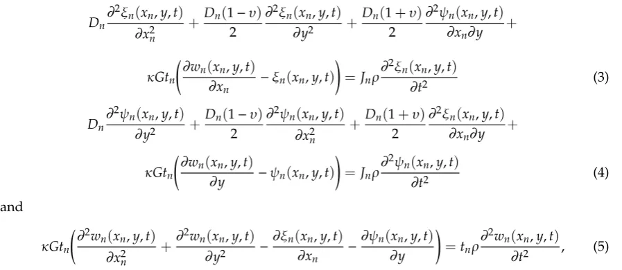
The equations modeling the out-of-plane motion of the components in the transverse z-direction are derived using Mindlin plate theory, and this set of equations is written as [4]

𝐷 𝜕 𝜉 (𝑥 , 𝑦, 𝑡)

𝜕𝑥 +

𝐷 (1 − 𝜐) 2

𝜕 𝜉 (𝑥 , 𝑦, 𝑡)

𝜕𝑦 +

𝐷 (1 + 𝜐) 2 𝜕 𝜓 (𝑥 , 𝑦, 𝑡) 𝜕𝑥 𝜕𝑦 + 𝜅𝐺𝑡 𝜕𝑤 (𝑥 , 𝑦, 𝑡) 𝜕𝑥 − 𝜉 (𝑥 , 𝑦, 𝑡) = 𝐽 𝜌 𝜕 𝜉 (𝑥 , 𝑦, 𝑡) 𝜕𝑡 (3) 𝐷 𝜕 𝜓 (𝑥 , 𝑦, 𝑡) 𝜕𝑦 +

𝐷 (1 − 𝜐) 2

𝜕 𝜓 (𝑥 , 𝑦, 𝑡)

𝜕𝑥 +

𝐷 (1 + 𝜐) 2 𝜕 𝜉 (𝑥 , 𝑦, 𝑡) 𝜕𝑥 𝜕𝑦 + 𝜅𝐺𝑡 𝜕𝑤 (𝑥 , 𝑦, 𝑡) 𝜕𝑦 − 𝜓 (𝑥 , 𝑦, 𝑡) = 𝐽 𝜌 𝜕 𝜓 (𝑥 , 𝑦, 𝑡) 𝜕𝑡 (4) and

𝜅𝐺𝑡 ( , , )+ ( , , )− ( , , )− ( , , ) = 𝑡 𝜌 ( , , ), (5)

where wn(xn,y,t) is the out-of-plane displacement, ξn(xn,y,t) is the angle of rotation of a normal line with respect to the y-coordinate, ψn(xn,y,t) is the angle of rotation of a normal line with respect to the

x-coordinate, κ is the shear correction factor, tn is the thickness, Dn is the flexural rigidity and is equal to

𝐷 = ₍ ₎. (6)

Jn is equal to

𝐽 = , (7)

and it is noted that tw = bw and tfl = tfr = hf.

The solutions to Equations (1) and (2) for the in-plane motion are [25]

𝑢 (𝑥 , 𝑦, 𝑡) = 𝑈 (𝑥 ) exp i𝑘 𝑦 exp(i𝜔𝑡) (8)

and

x_fl , u_fl y , v_fl

z_fl , w_fl

x_fr , u_fr y , v_fr

z_fr , w_fr z_w , w_w

y , v_w xw , uw

Left Flange Right Flange

Web

Figure 2.Model components and individual coordinate systems used in the analysis.

The equations modeling the out-of-plane motion of the components in the transversez-direction are derived using Mindlin plate theory, and this set of equations is written as [4]

Dn ∂2_ξ

n(xn,y,t)

∂x2 n

+Dn(1−υ)

2

∂2_ξ

n(xn,y,t)

∂y2 +

Dn(1+υ) 2

∂2_ψ

n(xn,y,t)

∂xn∂y

+

κGtn

∂wn(xn,y,t) ∂xn

−ξ_n₍_x_n_,_y_,_t₎

! =Jnρ

∂2_ξ

n(xn,y,t)

∂t2 (3)

Dn ∂2_ψ

n(xn,y,t)

∂y2 +

Dn(1−υ) 2

∂2_ψ

n(xn,y,t)

∂x2 n

+Dn(1+υ)

2

∂2_ξ

n(xn,y,t)

∂xn∂y

+

κGtn ∂

wn(xn,y,t)

∂y −ψn(xn,y,t)

! =Jnρ

∂2_ψ

n(xn,y,t)

∂t2 (4)

and

κGtn ∂ 2_w

n(xn,y,t)

∂x2n

+∂

2_w

n(xn,y,t)

∂y2 −

∂ξn(xn,y,t) ∂xn

−∂ψn(xn,y,t) ∂y

!

=tnρ∂ 2_w

n(xn,y,t)

∂t2 , (5) wherewn(xn,y,t) is the out-of-plane displacement,ξn(xn,y,t) is the angle of rotation of a normal line with respect to they-coordinate,ψn(xn,y,t) is the angle of rotation of a normal line with respect to the x-coordinate,κis the shear correction factor,tnis the thickness,Dnis the flexural rigidity and is equal to

Dn= Et3n

12(1−υ2₎. (6)

Jnis equal to

Jn = t 3 n

12, (7)

and it is noted thattw=bwandtfl=tfr=hf.

The solutions to Equations (1) and (2) for the in-plane motion are [25]

un(xn,y,t) =Un(xn)exp

ikyy

exp(iωt) (8)

and

vn(xn,y,t) =Vn(xn)exp

ikyy

(5)

Acoustics2019,1 730

where

Uw(xw) =C1αcos(αxw)−C2αsin(αxw) +C3ikysin(βxw) +C4ikycos(βxw) (10) Uf l

xf l

=C9αcos

αxf l

−_C₁₀α_sinα_x_{f l}₊_C₁₁_i_k_y_sinβ_x_{f l}₊_C₁₂_i_k_y_cosβ_x_{f l} ₍₁₁₎ Uf r

xf r

=C17αcos

αxf r

−_C₁₈α_sinα_x_{f r}₊_C₁₉_i_k_y_sinβ_x_{f r}₊_C₂₀_i_k_y_cosβ_x_{f r} ₍₁₂₎ Vw(xw) =C1ikysin(αxw) +C2ikycos(αxw)−C3βsin(βxw) +C4βcos(βxw) (13) Vf l

xf l

=C9ikysin

αxf l

+C10ikycos

αxf l

−_C₁₁β_cosβ_x_{f l}₊_C₁₂β_sinβ_x_{f l} ₍₁₄₎ Vf r

xf r

=C17ikysin

αxf r

+C18ikycos

αxf r

−_C₁₉β_cosβ_x_{f r}₊_C₂₀β_sinβ_x_{f r}_. ₍₁₅₎ In Equations (10)–(15),αandβare modified wavenumbers and are equal to

α= q

k2p−k2y (16)

and

β= q

k2s−k2y, (17)

wherekpis the plate wavenumber, expressed as kp= ω

cp

= _q ω

E

(1−υ2₎_ρ

, (18)

whereksis the shear wavenumber expressed as ks= ω

cs

= _qω

G

ρ

. (19)

The solutions town(xn,y,t) for Equations (3)–(5) for the out-of-plane motion are [25] wn(xn,y,t) =Wn(xn)exp

ikyy

exp(iωt), (20)

where

Ww(xw) =C5exp(λ1xw) +C6exp(λ2xw) +C7exp(λ3xw) +C8exp(λ4xw) (21) Wf l

xf l

=C13exp

λ5xf l

+C14exp

λ6xf l

+C15exp

λ7xf l

+C8exp

λ8xf l

(22)

and

Wf r

xf r

=C21exp

λ5xf r

+C22exp

λ6xf r

+C23exp

λ7xf r

+C24exp

λ8xf r

. (23)

In Equations (21)–(23), the values ofλiare out-of-plane eigenvalues and for Equation (21) are equal to [26]

λ1,2,3,4=±

s

−_b± √

b2−₄_ac

2a , (24)

where

a=DwκG (25)

b=−₂_D_wκ_Gk2

y+Dwρω2+JwκGρω2 (26)

c=DwκGk4y−Dwρω2k2y+JwκGρω2k2y+Jwρ2ω4−κGbwρω2 (27) and

λ5,6,7,8=±

s

−_b± √

b2−₄_ac

(6)

Acoustics2019,1 731

where

a=DfκG (29)

b=−₂_D_fκ_Gk2_y₊_D_fρω2₊_J_fκ_Gρω2 ₍₃₀₎ c=DfκGk4y−Dfρω2k2y+JfκGρω2k2y+Jfρ2ω4−κGhfρω2, (31) with

Df =Df l=Df r (32)

and

Jf =Jf l=Jf r. (33)

The solutions to the rotational angles are written as

ξn(xn,y,t) =Ξn(xn)exp

ikyy

exp(iωt) (34)

and

ψn(xn,y,t) =Ψn(xn)exp

ikyy

exp(iωt), (35)

where

Ξw(xw) =C5a1exp(λ1xw) +C6a2exp(λ2xw) +C7a3exp(λ3xw) +C8a4exp(λ4xw) (36)

Ξf l

xf l

=C13c1exp

λ5xf l

+C14c2exp

λ6xf l

+C15c3exp

λ7xf l

+C16c4exp

λ8xf l

(37)

Ξf r

xf r

=C21c1exp

λ5xf r

+C22c2exp

λ6xf r

+C23c3exp

λ7xf r

+C24c4exp

λ8xf r

(38)

Ψw(xw) =C5b1exp(λ1xw) +C6b2exp(λ2xw) +C7b3exp(λ3xw) +C8b4exp(λ4xw) (39)

Ψf l

xf l

=C13d1exp

λ5xf l

+C14d2exp

λ6xf l

+C15d3exp

λ7xf l

+C16d4exp

λ8xf l

(40)

and

Ψf r

xf r

=C21d1exp

λ5xf r

+C22d2exp

λ6xf r

+C23d3exp

λ7xf r

+C24d4exp

λ8xf r

, (41)

where

an= κGbwλn

Dwk2y−Dwλn2−Jwρω2+κGbw

(42)

bn=

κGbwiky

Dwk2y−Dwλn2−Jwρω2+κGbw

(43)

cn =

κGhfλ(n+4)

Dfk2y−Dfλ2₍_n₊₄₎−Jfρω2+κGhf

(44)

and

dn =

κGhfiky

Dfk2y−Dfλ2₍_n₊₄₎−Jfρω2+κGhf

. (45)

(7)

Acoustics2019,1 732

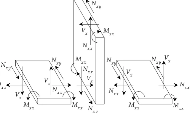
The various forces of the structure, shown in Figure3, are now mathematically defined. These will be used in the force and moment balance equations to solve for the values ofCi. The normal in-plane forces are determined using [27]

N(_xxn)(xn) = Etn 1−υ2

"

dUn(xn) dxn

+ikyυVn(xn)

#

(46)

and the shear in-plane forces are

Nxy(n)(xn) = Etn 2(1+υ)

"

ikyUn(xn) +

dVn(xn) dxn

#

. (47)

The shear out-of-plane forces are calculated using [26]

Vx(n)(xn) =κGtn

"

dWn(xn) dxn

−Ξ_n(xn)

#

+Dn(1−υ)

2

"

k2yΞn(xn)−ikydΨn

(xn) dxn

#

(48)

and the moments with respect to thex-axis are determined using

M(_xxn)(xn) =−Dn

"

dΞn(xn) dxn

+ikyυΨn(xn)

#

, (49)

where it is noted that the exponential terms exp(iωt) and exp(ikyy) are suppressed from Equations (46)–(49).

Acoustics 2019, 2 FOR PEER REVIEW 7

included here because they will be used to calculate the out-of-plane shear force and moment in the

x-direction.

The various forces of the structure, shown in Figure 3, are now mathematically defined. These will be used in the force and moment balance equations to solve for the values of Ci. The normal in-plane forces are determined using [27]

𝑁( )(𝑥 ) = 𝐸𝑡 1 − 𝜐

d𝑈 (𝑥 )

d𝑥 + i𝑘 𝜐𝑉 (𝑥 ) (46)

and the shear in-plane forces are

𝑁( )(𝑥 ) = ₍ ₎ i𝑘 𝑈 (𝑥 ) + ( ) . (47)

The shear out-of-plane forces are calculated using [26]

𝑉( )(𝑥 ) = 𝜅𝐺𝑡 d𝑊 (𝑥 )

d𝑥 − Ξ (𝑥 ) +

𝐷 (1 − 𝜐)

2 𝑘 Ξ (𝑥 ) − i𝑘

dΨ (𝑥 )

d𝑥 (48)

and the moments with respect to the x-axis are determined using

𝑀( )(𝑥 ) = −𝐷 ( )+ i𝑘 𝜐Ψ (𝑥 ), (49)

where it is noted that the exponential terms exp(iωt) and exp(ikyy) are suppressed from Equations (46)–(49).

Figure 3. Generalized forces on the boundaries of the system.

There are 24 boundary conditions on the beam. The boundary conditions at the top of the web (xw = hw) are

𝑁( )(ℎ ) = −𝑏 𝑃 (50)

𝑁( )(ℎ ) = −𝑏 𝐹 (51)

𝑉( )(ℎ ) = −𝑏 𝑄 (52)

and

𝑀( )(ℎ ) = 0, (53)

N_{x x} N_{x y}

V_x M_{x x}

N_{x x} N_{x y}

V_x

M_{x x} V_x

N_{x y} N_{x x} M_{x x}

V_x N_{x y}

N_{x x}

M_{x x}

N_{x x} N_{x y}

V_x

M_{x x}

N_{x x} N_{x y} Vx

M_{x x}

Figure 3.Generalized forces on the boundaries of the system.

There are 24 boundary conditions on the beam. The boundary conditions at the top of the web (xw=hw) are

N(xxn)(hw) =−bwP0 (50)

Nxy(n)(hw) =−bwF0 (51)

Vx(n)(hw) =−bwQ0 (52)

and

Mxx(n)(hw) =0, (53)

(8)

Acoustics2019,1 733

z-direction of the web. Implicit in these pressure loads is the multiplication of exponential functions in y-direction wavenumber and frequency. In general, the most important loading quantity is the normal pressure. Note that these forcing functions act on the top of the web, because this model allows the beam to be loaded at a location other than the neutral axis of the beam, and this corresponds more closely to the actual physical problem than loading the beam on its neutral axis. There are three force balances at the intersection of the web and flange (xw=xfl=xfr=0). These force balances are written as

Nxx(w)(0)−V

(f l)

x (0) +V

(f r)

x (0) =0 (54)

V_x(w)(0) +N_xx(f l)(0)−_N(f r)

xx (0) =0 (55)

N(xyw)(0)−N

(f l)

xy (0) +N

(f r)

xy (0) =0, (56)

and there is a moment balance at this location written as

M(xxw)(0)−M

(f l)

xx (0) +M

(f r)

xx (0) =0. (57)

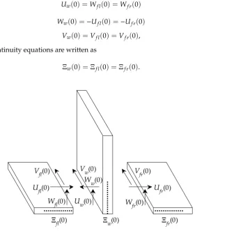
There are eight continuity equations for the intersection of the web and the flange. The continuity terms are shown in Figure4, and the displacement continuity equations are written as

Uw(0) =Wf l(0) =Wf r(0) (58) Ww(0) =−Uf l(0) =−Uf r(0) (59) Vw(0) =Vf l(0) =Vf r(0), (60) and the slope continuity equations are written as

Ξw(0) =Ξf l(0) =Ξf r(0). (61)

where P0 is the normal external pressure acting in the x-direction of the web, F0 is the axial external

pressure acting in the y-direction of the web, and Q0 is the transverse external pressure acting in the

z-direction of the web. Implicit in these pressure loads is the multiplication of exponential functions in y-direction wavenumber and frequency. In general, the most important loading quantity is the normal pressure. Note that these forcing functions act on the top of the web, because this model allows the beam to be loaded at a location other than the neutral axis of the beam, and this corresponds more closely to the actual physical problem than loading the beam on its neutral axis. There are three force balances at the intersection of the web and flange (xw = xfl = xfr = 0). These force balances are written as

𝑁( )(0) − 𝑉( )(0) + 𝑉( )(0) = 0 (54)

𝑉( )(0) + 𝑁( )(0) − 𝑁( )(0) = 0 (55)

𝑁( )(0) − 𝑁( )(0) + 𝑁( )(0) = 0, (56)

and there is a moment balance at this location written as

𝑀( )(0) − 𝑀( )(0) + 𝑀( )(0) = 0. (57)

There are eight continuity equations for the intersection of the web and the flange. The continuity terms are shown in Figure 4, and the displacement continuity equations are written as

𝑈 (0) = 𝑊 (0) = 𝑊 (0) (58)

𝑊 (0) = −𝑈 (0) = −𝑈 (0) (59)

𝑉 (0) = 𝑉 (0) = 𝑉 (0), (60)

and the slope continuity equations are written as

Ξ (0) = Ξ (0) = Ξ (0). (61)

Figure 4. Continuity terms at the intersection of the web and flange.

The boundary conditions at the free end of the left flange (xfl = a) are

𝑁( )(𝑎) = 0 (62)

V_fl(0) Vw(0) V_fr(0)

U_fl(0)

W_w(0)

U_fr(0)

W_fl(0) U_w(0) W_fr(0)

Ξ_fl(0) Ξ_w(0) Ξ_fr(0)

Figure 4.Continuity terms at the intersection of the web and flange.

The boundary conditions at the free end of the left flange (xfl=a) are

N_xx(f l)(a) =0 (62)

(9)

Acoustics2019,1 734

V(_xf l)(a) =0 (64)

and

M(xxf l)(a) =0, (65)

where it is noted thata<0. The boundary conditions at the free end of the right flange (xfr=b) are

Nxx(f r)(b) =0 (66)

N_xy(f r)(b) =0 (67)

V_x(f r)(b) =0 (68)

and

M(xxf r)(b) =0. (69)

Inserting Equations (10)–(15), (21)–(23), and (36)–(41) into Equations (50)–(69) produces a 24-by-24 algebraic matrix equation given by

[A]{_x}₌{_b}_, ₍₇₀₎

where the entries of [A] are in the AppendixAas Equations (A1)–(A132), the vector {x} is

{_x}₌n _C₁ _C₂ . . . _C₂₃ _C₂₄ oT ₍₇₁₎ and the {b} vector is

{_b}₌n −_b_w_P₀ −_b_w_F₀ −_b_w_Q₀ ₀ ₀ . . . ₀ ₀ oT_. ₍₇₂₎ The solution to the wave propagation coefficientsCiin Equation (70) is found using

{_x}= [A]−1{_b}_. ₍₇₃₎

Once these coefficients are known, they can be inserted into Equations (10), (13), and (21), and the response of the web for external loading in three dimensions can be calculated. Additionally, the displacement of the flange can also be calculated, but it is typically not a quantity of interest.

To integrate this beam model into a reinforced structural model, the dynamic stiffness components of the beam are typically calculated and used. For a symmetric T-beam, there are four unique and nonzero terms. The first term is the dynamic stiffness of the normal displacement to normal pressure and is written as

Kzz=

−_b_w_P₀ Uw(hw)

; (74)

the second term is the dynamic stiffness of normal displacement to axial pressure (and equal to axial displacement to normal pressure) and is written as

Kzy =Kyz=

−_b_w_F₀ Uw(hw)

= −bwP0

Vw(hw)

; (75)

the third term is the dynamic stiffness of axial displacement to axial pressure and is written as

Kyy= −_b_w_F₀ Vw(hw)

(10)

Acoustics2019,1 735

and the fourth term is the dynamic stiffness of transverse displacement to transverse pressure and is written as

Kxx =

−_b_w_Q₀ Ww(hw)

, (77)

where the units of Equations (74)–(77) are stiffness per unit length, which in the metric system is (N/m)/m or alternatively N·_m−₂

. Finally, it is noted that, if a second flange is present on the top of the beam, i.e., an I- or an H-beam design, this dynamic contribution can be added to the model in the same method as the bottom flange equations.

3. Results

The model is now analyzed using an example problem where the beam has material and geometric properties that are consistent with an application in underwater structures. The T-beam has the following physical dimensions: height of the web hw = 0.2436 m (9.59 in), width of the webbw=0.0140 m (0.550 in), height of the flangehf=0.0333 m (1.310 in), and width of the flange bf=0.1981 m (7.800 in), which results ina=−0.0991 m andb=0.0991 m. The beam is made of steel that has the following mechanical properties: Young’s modulusE=200×₁₀9_N·_m−2_{, shear modulus} G=76.92×₁₀9_N·_m−2_{, Poisson’s ratio}υ=_{0.30, and density}ρ=_{7800 kg}·_m−3_{. The value for the shear} correction factor isκ=0.8333. The analytical model was programmed and the results were displayed using the MATLAB programming language.

The beam is independently loaded on its top surface with three separate loads that correspond to normal (web in-plane), axial (web in-plane) and transverse (web out-of-plane) pressure. Although any location of the beam can be chosen for displacement output, the top of the web is investigated here because this location is pertinent to the analysis of reinforced structures. This allows the dynamic stiffness of the beam to be calculated and subsequently used in analysis of beams attached to plates or elastic bodies. Thus, the output of the model is normal, axial, and transverse beam displacement at the top of the web. It is noted, however, that by far the most important model output is the normal displacement divided by normal pressure as this corresponds to the main design objective of most beams. Plots of the other outputs are included for completeness. The finite element model results were produced using COMSOL finite element program using a model that consisted of 2200 quadratic serendipity hexahedral elements and a total of 49,659 degrees of freedom.

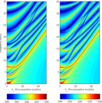
Figure5is a comparison of the normal displacement divided by the normal pressure versus the axial wavenumber and frequency in the decibel scale referenced to m Pa−1. The analytical model results are on the left and the finite element results are on the right. Figure6is a plot of the normal beam stiffnessKzzversus frequency at zero axial wavenumber in the decibel scale referenced to (N/m)/m. The analytical model is the solid line, the previous analytical model [1,2] are the square markers, the Timoshenko beam model [6] are the diamond markers and the finite element results are depicted with circular markers. The Timoshenko beam stiffness in the normal direction was calculated using the following equation [6]:

Kzz

ky≡0

= AIρ

2_ω4₋_A2_κ_G_ρω2

AκG−_Iρω2 , (78)

whereAis the area, andIis the area moment of inertia of the T-beam incorporating both the web and the flange components as a single entity. These values areA=0.01 m2, andI=6.044×₁₀−₅

(11)

Acoustics2019,1 736

displacement divided by the normal pressure versus the axial wavenumber and frequency. Note that Figure11is also identical to the normal displacement divided by the axial pressure. The beam transfer functions of normal displacement divided by axial forcing and axial displacement divided by normal forcing are both zero for zero axial wavenumber; thus, the beam stiffness termsKzyandKzyhave no physical meaning (forky=0 only), and these quantities do not have corresponding stiffness plots. Note that in Figure5through Figure11there is broad-based agreement between the new analytical model and the finite element model. Additionally, the Timoshenko beam model in Figure6is valid to approximately 1 kHz, where the magnitude begins to diverge from both the analytical models and the finite element model.

model in Figure 6 is valid to approximately 1 kHz, where the magnitude begins to diverge from both the analytical models and the finite element model.

Figure 5. Normal displacement divided by normal force versus wavenumber and frequency in decibels referenced to m·Pa−1_{. The analytical model results are on the left and the finite element results} are on the right.

Figure 6. Magnitude of normal beam stiffness Kzzversus frequency at zero axial wavenumber. The

analytical model is the solid line, the previous analytical model [1,2] are the square markers, the Timoshenko beam model [6] are the diamond markers and the finite element results are depicted with circular markers.

k_y Wavenumber (rad/m)

Fr

equ

en

cy

(

k

H

z

)

0 20 40

0 5 10 15 20 25 30 35

-280 -260 -240 -220 -200

0 20 40

5 10 15 20 25 30 35

-280 -260 -240 -220 -200

0 5 10 15 20 25 30 35

180 200 220 240 260

Frequency (kHz)

Ma

gn

it

u

d

e

K zz

(

d

B

r

ef (N

/m

)/

m

)

(12)

Acoustics2019,1 737 Acoustics 2019, 2 FOR PEER REVIEW 11

model in Figure 6 is valid to approximately 1 kHz, where the magnitude begins to diverge from both the analytical models and the finite element model.

Figure 5. Normal displacement divided by normal force versus wavenumber and frequency in decibels referenced to m·Pa−1_{. The analytical model results are on the left and the finite element results} are on the right.

Figure 6. Magnitude of normal beam stiffness Kzzversus frequency at zero axial wavenumber. The

analytical model is the solid line, the previous analytical model [1,2] are the square markers, the Timoshenko beam model [6] are the diamond markers and the finite element results are depicted with circular markers.

Fr

equ

en

cy

(

k

H

z

)

0 20 40

0 5 10 15 20 25 30 35

-280 -260 -240 -220 -200

0 20 40

5 10 15 20 25 30 35

-280 -260 -240 -220 -200

0 5 10 15 20 25 30 35

180 200 220 240 260

Frequency (kHz)

Ma

gn

it

u

d

e

K zz

(

d

B

r

ef (N

/m

)/

m

)

Figure 6.Magnitude of normal beam stiffnessKzzversus frequency at zero axial wavenumber. The analytical model is the solid line, the previous analytical model [1,2] are the square markers, the Timoshenko beam model [6] are the diamond markers and the finite element results are depicted with circular markers.

Figure 7. Axial displacement divided by axial force versus wavenumber and frequency in decibels referenced to m Pa−1_{. The analytical model results are on the left and the finite element results are on} the right.

Figure 8. Magnitude of axial beam stiffness Kyy versus frequency at zero axial wavenumber. The

analytical model is the solid line, the previous analytical model [1,2] are the square markers and the finite element results are depicted with circular markers.

Frequ

en

cy

(

k

H

z

)

0 20 40

0 5 10 15 20 25 30 35

-280 -260 -240 -220 -200

0 20 40

5 10 15 20 25 30 35

-280 -260 -240 -220 -200

0 5 10 15 20 25 30 35

180 200 220 240 260

Frequency (kHz)

Ma

gn

it

u

d

e

K yy

(d

B

r

ef

(N

/m

)/

m

)

Figure 7. Axial displacement divided by axial force versus wavenumber and frequency in decibels referenced to m Pa−1_{. The analytical model results are on the left and the finite element results are on}

(13)

Figure 7. Axial displacement divided by axial force versus wavenumber and frequency in decibels referenced to m Pa−1_{. The analytical model results are on the left and the finite element results are on} the right.

Figure 8. Magnitude of axial beam stiffness Kyy versus frequency at zero axial wavenumber. The

analytical model is the solid line, the previous analytical model [1,2] are the square markers and the finite element results are depicted with circular markers.

Frequ

en

cy

(

k

H

z

)

0 20 40

0 5 10 15 20 25 30 35

-280 -260 -240 -220 -200

0 20 40

5 10 15 20 25 30 35

-280 -260 -240 -220 -200

0 5 10 15 20 25 30 35

180 200 220 240 260

Frequency (kHz)

Ma

gn

it

u

d

e

K yy

(d

B

r

ef

(N

/m

)/

m

)

Figure 8. Magnitude of axial beam stiffnessKyy versus frequency at zero axial wavenumber. The analytical model is the solid line, the previous analytical model [1,2] are the square markers and the finite element results are depicted with circular markers.

Figure 9. Transverse displacement divided by transverse force versus wavenumber and frequency in decibels referenced to m Pa−1_{. The analytical model results are on the left and the finite element results} are on the right.

Figure 10. Magnitude of transverse beam stiffness Kxxversus frequency at zero axial wavenumber.

The analytical model is the solid line, the previous analytical model [1,2] are the square markers and the finite element results are depicted with circular markers.

Frequ

en

cy

(

k

H

z

)

0 20 40

0 5 10 15 20 25 30 35

-260 -240 -220 -200 -180

0 20 40

5 10 15 20 25 30 35

-260 -240 -220 -200 -180

0 5 10 15 20 25 30 35

160 180 200 220 240

Frequency (kHz)

Ma

gn

it

u

d

e

K xx

(

d

B

r

ef (N

/m

)/

m

)

(14)

Figure 9. Transverse displacement divided by transverse force versus wavenumber and frequency in decibels referenced to m Pa−1_{. The analytical model results are on the left and the finite element results} are on the right.

Figure 10. Magnitude of transverse beam stiffness Kxxversus frequency at zero axial wavenumber.

The analytical model is the solid line, the previous analytical model [1,2] are the square markers and the finite element results are depicted with circular markers.

Frequ

en

cy

(

k

H

z

)

0 20 40

0 5 10 15 20 25 30 35

-260 -240 -220 -200 -180

0 20 40

5 10 15 20 25 30 35

-260 -240 -220 -200 -180

0 5 10 15 20 25 30 35

160 180 200 220 240

Frequency (kHz)

Ma

gn

it

u

d

e

K xx

(

d

B

r

ef (N

/m

)/

m

)

Figure 10. Magnitude of transverse beam stiffnessKxxversus frequency at zero axial wavenumber. The analytical model is the solid line, the previous analytical model [1,2] are the square markers and the finite element results are depicted with circular markers.

Figure 11. Axial displacement divided by normal force versus wavenumber and frequency in decibels referenced to m Pa−1_{. The analytical model results are on the left and the finite element results are on} the right.

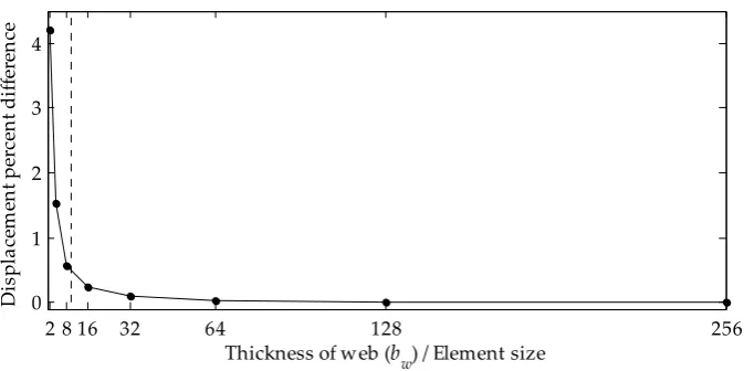
To ensure the finite element results have accurately converged, the finite element model was rerun at a frequency of 35 kHz and a wavenumber of 50 rad·m−1_{with various sized elements. The}

previous results were generated with a web thickness (bw) divided by element size ratio of 10. This ratio was changed to 1, 2, 4, 8, 16, 64, 128 and 256 and a comparison of the web normal displacement at each ratio was compared to the web normal displacement at a ratio of 256. It was found that using a ratio of 10 produced results that had approximately a 0.4% difference (−8 dB) compared to a mesh size that was 10 times more dense. These convergence results are shown graphically in Figure 12 where the dashed line corresponds to the finite element results presented in this section.

Frequ

en

cy

(

k

H

z

)

0 20 40

0 5 10 15 20 25 30 35

-280 -260 -240 -220 -200

0 20 40

5 10 15 20 25 30 35

-280 -260 -240 -220 -200

Figure 11.Axial displacement divided by normal force versus wavenumber and frequency in decibels referenced to m Pa−1. The analytical model results are on the left and the finite element results are on the right.

To ensure the finite element results have accurately converged, the finite element model was rerun at a frequency of 35 kHz and a wavenumber of 50 rad·_m−₁

(15)

Acoustics2019,1 740

changed to 1, 2, 4, 8, 16, 64, 128 and 256 and a comparison of the web normal displacement at each ratio was compared to the web normal displacement at a ratio of 256. It was found that using a ratio of 10 produced results that had approximately a 0.4% difference (−_{8 dB) compared to a mesh size that} was 10 times more dense. These convergence results are shown graphically in Figure12where the dashed line corresponds to the finite element results presented in this section.Acoustics 2019, 2 FOR PEER REVIEW 15

Figure 12. Web normal displacement percent difference versus thickness of web divided by element size. The dashed line corresponds to finite element results presented herein and the percent difference is 0.4% compared to a model with a grid approximately 25 times more dense.

The beam system presented here supports an infinite number of propagating modes that are illustrated in Figures 5, 7, 9 and 11 as high-displacement regions. Because the most important response of the system is the normal displacement divided by the normal pressure, the first four dominant modes from this transfer function near zero axial wavenumber are plotted. Figure 13 is a plot of the mode shape at 202 Hz, Figure 14 is a plot of the mode shape at 3305 Hz, Figure 15 is a plot of the mode shape at 7228 Hz, and Figure 16 is a plot of the mode shape at 15,036 Hz. In Figures 13 through 16, the left portion of the plots are the axial displacements and the right portion are the normal displacements. The transverse displacements for these modes are zero or very close to zero and are not shown. The mode shapes are symmetric about the web, i.e., the right flange response will be identical to the response of the left flange. In all of the plots, the axial wavenumber was set equal to 2 rad m−1_{as a value of zero will yield an axial displacement of zero everywhere. The first mode}

shape is a low-frequency flexural wave whereas the others are more complex in their displacement shapes and are based on the geometric properties of the web and flange. Note that the beam stiffness

Kzz is zero at these resonant frequency locations.

Figure 13. Plot of the first mode shape at 202 Hz, where the axial displacement is on the left and the normal displacement is on the right.

2 8 16 32 64 128 256

0 1 2 3 4

Thickness of web (b_w) / Element size

D

is

p

la

ce

m

en

t p

erc

en

t d

if

fe

ren

ce

V_w(x_w)

V_fl(x_fl)

U_w(x_w)

W_fl(x_fl)

Figure 12.Web normal displacement percent difference versus thickness of web divided by element size. The dashed line corresponds to finite element results presented herein and the percent difference is 0.4% compared to a model with a grid approximately 25 times more dense.

The beam system presented here supports an infinite number of propagating modes that are illustrated in Figures5,7,9and11, Figure7as high-displacement regions. Because the most important response of the system is the normal displacement divided by the normal pressure, the first four dominant modes from this transfer function near zero axial wavenumber are plotted. Figure13is a plot of the mode shape at 202 Hz, Figure14is a plot of the mode shape at 3305 Hz, Figure15is a plot of the mode shape at 7228 Hz, and Figure16is a plot of the mode shape at 15,036 Hz. In Figures13–16, the left portion of the plots are the axial displacements and the right portion are the normal displacements. The transverse displacements for these modes are zero or very close to zero and are not shown. The mode shapes are symmetric about the web, i.e., the right flange response will be identical to the response of the left flange. In all of the plots, the axial wavenumber was set equal to 2 rad m−₁

(16)

Figure 12. Web normal displacement percent difference versus thickness of web divided by element size. The dashed line corresponds to finite element results presented herein and the percent difference is 0.4% compared to a model with a grid approximately 25 times more dense.

The beam system presented here supports an infinite number of propagating modes that are illustrated in Figures 5, 7, 9 and 11 as high-displacement regions. Because the most important response of the system is the normal displacement divided by the normal pressure, the first four dominant modes from this transfer function near zero axial wavenumber are plotted. Figure 13 is a plot of the mode shape at 202 Hz, Figure 14 is a plot of the mode shape at 3305 Hz, Figure 15 is a plot of the mode shape at 7228 Hz, and Figure 16 is a plot of the mode shape at 15,036 Hz. In Figures 13 through 16, the left portion of the plots are the axial displacements and the right portion are the normal displacements. The transverse displacements for these modes are zero or very close to zero and are not shown. The mode shapes are symmetric about the web, i.e., the right flange response will be identical to the response of the left flange. In all of the plots, the axial wavenumber was set equal to 2 rad m−1_{as a value of zero will yield an axial displacement of zero everywhere. The first mode}

shape is a low-frequency flexural wave whereas the others are more complex in their displacement shapes and are based on the geometric properties of the web and flange. Note that the beam stiffness

Kzz is zero at these resonant frequency locations.

Figure 13. Plot of the first mode shape at 202 Hz, where the axial displacement is on the left and the normal displacement is on the right.

2 8 16 32 64 128 256

0 1 2 3 4

Thickness of web (b_w) / Element size

D

is

p

la

ce

m

en

t p

erc

en

t d

if

fe

ren

ce

V_w(x_w)

V_fl(x_fl)

U_w(x_w)

W_fl(x_fl)

Figure 13.Plot of the first mode shape at 202 Hz, where the axial displacement is on the left and the normal displacement is on the right.

Figure 14. Plot of the second mode shape at 3305 Hz where the axial displacement is on the left and the normal displacement is on the right.

Figure 15. Plot of the third mode shape at 7228 Hz, where the axial displacement is on the left and the normal displacement is on the right.

Figure 16. Plot of the third mode shape at 15,036 Hz, where the axial displacement is on the left and the normal displacement is on the right.

V_w(x_w)

V_fl(x_fl)

U_w(x_w)

W_fl(x_fl)

V_w(x_w)

V_fl(x_fl)

U_w(x_w)

W_fl(x_fl)

V_w(x_w)

V_fl(x_fl)

U_w(x_w)

W_fl(x_fl)

Figure 14.Plot of the second mode shape at 3305 Hz where the axial displacement is on the left and the normal displacement is on the right.

V_w(x_w)

V_fl(x_fl)

U_w(x_w)

W_fl(x_fl)

V_w(x_w)

V_fl(x_fl)

U_w(x_w)

W_fl(x_fl)

V_w(x_w)

V_fl(x_fl)

U_w(x_w)

W_fl(x_fl)

(17)

V_w(x_w)

V_fl(x_fl)

U_w(x_w)

W_fl(x_fl)

V_w(x_w)

V_fl(x_fl)

U_w(x_w)

W_fl(x_fl)

V_w(x_w)

V_fl(x_fl)

U_w(x_w)

W_fl(x_fl)

Figure 16.Plot of the third mode shape at 15,036 Hz, where the axial displacement is on the left and the normal displacement is on the right.

4. Conclusions

A high-frequency analytical model for a T-shaped beam was derived and compared to a previous analytical model, a Timoshenko beam model, and a fully elastic finite element model. This new model was constructed with two-dimensional elastic equations for the in-plane motion and Mindlin plate equations for the out-of-plane motion. This allows for almost a total elastic response of the entire system. For the beam example problem presented, the analytical model and the finite element compared favorably up to 35 kHz. Four of the mode shapes of the beam were plotted. The application of this model to a reinforced structure is discussed.

Author Contributions: Individual contributions are as follows: Conceptualization, A.J.H., D.P. and D.L.C.; analytical software, A.J.H.; finite element software, D.P. and D.L.C.; validation, A.J.H., D.P. and D.L.C.; writing—original draft preparation, A.J.H.; writing—review and editing, A.J.H., D.P. and D.L.C.; and funding acquisition, A.J.H.

Funding: This work was funded by the Naval Undersea Warfare Center (NUWC) In-House Laboratory Independent Research (ILIR) Program.

Acknowledgments:The authors wish to thank Anthony A. Ruffa of NUWC Chief Technology Office (CTO).

Conflicts of Interest:The authors declare no conflicts of interest. The funding sponsors had no role in the design of the study; in the collection, analyses, or interpretation of data; in the writing of the manuscript, and in the decision to publish the results.

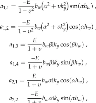
Appendix A

The nonzero entries to the [A] matrix in Equation (70) are listed in this appendix.

a1,1= −_E 1−υ2bw

α2₊_υ_k2 y

sin(αhw), (A1)

a1,2 = −_E 1−υ2bw

α2₊_υ_k2 y

cos(αhw), (A2)

a1,3 = E

1+υbwβikycos(βhw), (A3)

a1,4 = −_E

1+υbwβikysin(βhw), (A4)

a2,1= E

1+υbwαikycos(αhw), (A5)

a2,2= −_E

(18)

Acoustics2019,1 743

a2,3= E 2(1+υ)bw

β2₋_k2 y

sin(βhw), (A7)

a2,4= E 2(1+υ)bw

β2₋_k2 y

cos(βhw), (A8)

a3,5 =

     

Dwa1k2y(1−υ)

2 −

Dwb1ikyλ1(1−υ)

2 −κGbw(a1−λ1)

     exp

(λ₁hw), (A9)

a3,6 =

     

Dwa2k2y(1−υ)

2 −

Dwb2ikyλ2(1−υ)

     exp

(λ2hw), (A10)

a3,7 =

     

Dwa3k2y(1−υ)

2 −

Dwb3ikyλ3(1−υ)

    

exp(λ3hw), (A11)

a3,8 =

     

Dwa4k2y(1−υ)

2 −

Dwb4ikyλ4(1−υ)

     exp

(λ₄hw), (A12)

a4,5 =−Dw

a1λ1+b1ikyυ

exp(λ₁hw), (A13) a4,6 =−Dw

a2λ2+b2ikyυ

exp(λ2hw), (A14) a4,7 =−Dw

a3λ3+b3ikyυ

exp(λ₃hw), (A15) a4,8 =−Dw

a4λ4+b4ikyυ

exp(λ4hw), (A16) a5,2=

−_E 1−υ2bw

α2₊_υ_k2 y

, (A17)

a5,3= E

1+υbwβiky, (A18)

a5,13=

−_D_f_c₁_k2

y(1−υ)

2 +

Dfd1ikyλ5(1−υ)

2 +κGhf(c1−λ5), (A19) a5,14=

−_D_f_c₂_k2

y(1−υ)

2 +

Dfd2ikyλ6(1−υ)

2 +κGhf(c2−λ6), (A20) a5,15=

−_D_f_c₃_k2_y(1−υ)

2 +

Dfd3ikyλ7(1−υ)

2 +κGhf(c3−λ7), (A21) a5,16=

−_D_f_c₄_k2_y(1−υ)

2 +

Dfd4ikyλ8(1−υ)

2 +κGhf(c4−λ8), (A22) a5,21=

Dfc1k2y(1−υ)

2 −

Dfd1ikyλ5(1−υ)

2 −κGhf(c1−λ5), (A23) a5,22=

Dfc2k2y(1−υ)

2 −

Dfd2ikyλ6(1−υ)

2 −κGhf(c2−λ6), (A24) a5,23=

Dfc3k2y(1−υ)

2 −

Dfd3ikyλ7(1−υ)

2 −κGhf(c3−λ7), (A25) a5,24=

Dfc4k2y(1−υ)

2 −

Dfd4ikyλ8(1−υ)

2 −κGhf(c4−λ8), (A26) a6,5=

Dwa1k2y(1−υ)

2 −

Dwb1ikyλ1(1−υ)

2 −κGbw(a1−λ1), (A27) a6,6=

Dwa2k2y(1−υ)

2 −

Dwb2ikyλ2(1−υ)

(19)

Acoustics2019,1 744

a6,7=

Dwa3k2y(1−υ)

2 −

Dwb3ikyλ3(1−υ)

2 −κGbw(a3−λ3), (A29) a6,8=

Dwa4k2y(1−υ)

2 −

Dwb4ikyλ4(1−υ)

2 −κGbw(a4−λ4), (A30) a6,10=

−_E 1−υ2hf

α2₊_υ_k2 y

, (A31)

a6,11= E

1+υhfβiky, (A32)

a6,18= E 1−υ2hf

α2₊_υ_k2 y

, (A33)

a6,19= −_E

1+υhfβiky, (A34)

a7,1= E

1+υbwαiky, (A35)

a7,4= E 2(1+υ)bw

β2₋_k2 y

, (A36)

a7,9= −_E

1+υhfαiky, (A37)

a7,12= −_E 2(1+υ)hf

β2₋_k2 y

, (A38)

a7,17= E

1+υhfαiky, (A39)

a7,20= E 2(1+υ)hf

β2₋_k2 y

, (A40)

a8,5=−Dw

a1λ1+b1ikyυ

, (A41)

a8,6=−Dw

a2λ2+b2ikyυ

, (A42)

a8,7=−Dw

a3λ3+b3ikyυ

, (A43)

a8,8=−Dw

a4λ4+b4ikyυ

, (A44)

a8,13=Df

c1λ5+d1ikyυ

, (A45)

a8,14=Df

c2λ6+d2ikyυ

, (A46)

a8,15=Df

c3λ7+d3ikyυ

, (A47)

a8,16=Df

c4λ8+d4ikyυ

, (A48)

a8,21=−Df

c1λ5+d1ikyυ

, (A49)

a8,22=−Df

c2λ6+d2ikyυ

, (A50)

a8,23=−Df

c3λ7+d3ikyυ

, (A51)

a8,24=−Df

c4λ8+d4ikyυ

, (A52)

a9,1=α, (A53)

(20)

Acoustics2019,1 745

a9,13=−1 , (A55)

a9,14=−1 , (A56)

a9,15=−1 , (A57)

a9,16=−1 , (A58)

a10,1=α, (A59)

a10,4=iky, (A60)

a10,21=−1 , (A61)

a10,22=−1 , (A62)

a10,23=−1 , (A63)

a10,24=−1 , (A64)

a11,5=1 , (A65)

a11,6=1 , (A66)

a11,7=1 , (A67)

a11,8=1 , (A68)

a11,9=α, (A69)

a11,12=iky, (A70)

a12,5=1 , (A71)

a12,6=1 , (A72)

a12,7=1 , (A73)

a12,8=1 , (A74)

a12,17=α, (A75)

a12,20=iky, (A76)

a13,2=iky, (A77)

a13,3=−β, (A78)

a13,10=−iky, (A79)

a13,11=β, (A80)

a14,2=iky, (A81)

a14,3=−β, (A82)

a14,18=−iky, (A83)

a14,19=β, (A84)

a15,5=a1, (A85)

a15,6=a2, (A86)

a15,7=a3, (A87)

(21)

Acoustics2019,1 746

a15,13=−c1, (A89)

a15,14=−c2, (A90)

a15,15=−c3, (A91)

a15,16=−c4, (A92)

a16,5=a1, (A93)

a16,6=a2, (A94)

a16,7=a3, (A95)

a16,8=a4, (A96)

a16,21=−c1, (A97)

a16,22=−c2, (A98)

a16,23=−c3, (A99)

a16,24=−c4, (A100)

a17,9= −_E 1−υ2hf

α2₊_υ_k2 y

sin(αa), (A101)

a17,10= −_E 1−υ2hf

α2₊_υ_k2 y

cos(αa), (A102)

a17,11= E

1+υhfβikycos(βa), (A103)

a17,12= −_E

1+υhfβikysin(βa), (A104)

a18,9= E

1+υhfαikycos(αa), (A105)

a18,10= −_E

1+υhfαikysin(αa), (A106)

a18,11= E 2(1+υ)hf

β2₋_k2 y

sin(βa), (A107)

a18,12= E 2(1+υ)hf

β2₋_k2 y

cos(βa), (A108)

a19,13=

     

Dfc1k2y(1−υ)

2 −

Dfd1ikyλ5(1−υ)

2 −κGhf(c1−λ5)

    

exp(λ5a), (A109)

a19,14=



    

Dfc2k2y(1−υ)

2 −

Dfd2ikyλ6(1−υ)



   

exp

(λ₆a), (A110)

a19,15=

     

Dfc3k2y(1−υ)

2 −

Dfd3ikyλ7(1−υ)

    

exp

(λ7a), (A111)

a19,16=

     

Dfc4k2y(1−υ)

2 −

Dfd4ikyλ8(1−υ)

    

exp(λ8a), (A112)

a20,13=−Df

c1λ5+d1ikyυ

exp(λ5a), (A113) a20,14=−Df

c2λ6+d2ikyυ

(22)

Acoustics2019,1 747

a20,15=−Df

c3λ7+d3ikyυ

exp(λ₇a), (A115) a20,16=−Df

c4λ8+d4ikyυ

exp(λ8a), (A116) a21,17=

−_E 1−υ2hf

α2₊_υ_k2 y

sin(αb), (A117)

a21,18= −_E 1−υ2hf

α2₊_υ_k2 y

cos(αb), (A118)

a21,19= E

1+υhfβikycos(βb), (A119)

a21,20= −_E

1+υhfβikysin(βb), (A120)

a22,17= E

1+υhfαikycos(αb), (A121)

a22,18= −_E

1+υhfαikysin(αb), (A122)

a22,19= E 2(1+υ)hf

β2₋_k2 y

sin(βb), (A123)

a22,20= E 2(1+υ)hf

β2₋_k2 y

cos(βb), (A124)

a23,21=

     

Dfc1k2y(1−υ)

2 −

Dfd1ikyλ5(1−υ)

     exp

(λ₅b), (A125)

a23,22=

     

Dfc2k2y(1−υ)

2 −

Dfd2ikyλ6(1−υ)

     exp

(λ6b), (A126)

a23,23=

     

Dfc3k2y(1−υ)

2 −

Dfd3ikyλ7(1−υ)

    

exp(λ7b), (A127)

a23,24=

     

Dfc4k2y(1−υ)

2 −

Dfd4ikyλ8(1−υ)

     exp

(λ₈b), (A128)

a24,21=−Df

c1λ5+d1ikyυ

exp(λ₅b), (A129) a24,22=−Df

c2λ6+d2ikyυ

exp(λ6b), (A130) a24,23=−Df

c3λ7+d3ikyυ

exp(λ₇b), (A131) and

a24,24=−Df

c4λ8+d4ikyυ

exp(λ8b). (A132) References

1. Hull, A.J.; Perez, D.; Cox, D.L.A Hybrid T Beam Model in a Cartesian Coordinate System; NUWC-NPT Technical Memorandum 17-020; Naval Undersea Warfare Center Division: Newport, RI, USA, 15 March 2017. 2. Hull, A.J.; Perez, D.; Cox, D.L. A comprehensive analytical dynamic model of a T-beam.Int. J. Acoust. Vib.

2019,24, 139–149. [CrossRef]

3. Love, A.E.H. On the small free vibrations and deformations of elastic shells.Philos. Trans. R. Soc. Lond. 1888, 179, 491–549. [CrossRef]

(23)

Acoustics2019,1 748

5. Han, S.M.; Benaroya, H.; Wei, T. Dynamics of transversely vibrating beams using four engineering theories. J. Sound Vib.1999,225, 935–988. [CrossRef]

6. Timoshenko, S.P. On the transverse vibrations of bars of uniform cross-section.Lond. Edinb. Dublin Philos. Mag. J. Sci.1922,43, 125–131. [CrossRef]

7. Bickford, W.B. A Consistent Higher Order Beam Theory. In Proceedings of the 11th Southeastern Conference on Theoretical and Applied Mechanics, Huntsville, AL, USA, 8–9 April 1982; pp. 137–150.

8. Karama, M.; Afaq, K.S.; Mistou, S. Mechanical behavior of laminated composite beam by new multi-layered laminated composite structures model with transverse shear stress continuity.Int. J. Solids Struct.2003,40, 1525–1546. [CrossRef]

9. Reddy, J.N.; Phan, N.D. Stability and vibration of isotropic, orthotropic and laminated plates according to a higher-order shear deformation theory.J. Sound Vib.1985,98, 157–170. [CrossRef]

10. Park, D.-H.; Hong, S.-Y.; Kil, H.-G.; Jeon, J.-J. Power flow models and analysis of in-plane waves in finite coupled thin plates.J. Sound Vib.2001,244, 651–668. [CrossRef]

11. Kessissoglou, N.J. Power transmission in L-shaped plates including flexural and in-plane vibration.J. Acoust. Soc. Am.2004,115, 1157–1169. [CrossRef]

12. Du, J.; Li, W.L.; Liu, Z.; Yang, T.; Jin, G. Free vibration of two elastically coupled rectangular plates with uniform elastic boundary restraints.J. Sound Vib.2011,330, 788–804. [CrossRef]

13. Chen, Y.; Jin, G.; Zhu, M.; Liu, Z.; Du, J.; Li, W.L. Vibration behaviors of a box-type structure built up by plates and energy transmission through the structure.J. Sound Vib.2012,331, 849–867. [CrossRef]

14. Wang, X. Dynamic behavior of finite coupled Mindlin plates with a blocking mass. ASME J. Vib. Acoust.

2016,138, 061008. [CrossRef]

15. Abdul-Ahad, R.B.; Aziz, O.Q. Flexural strength of reinforced concrete T-Beams with steel fibers.Cem. Concr. Compos.1999,21, 263–268. [CrossRef]

16. Rahal, K. Combined torsion and bending in reinforced and prestressed concrete beams using simplified method for combined stress-resultants.Aci Struct. J.2007,104, 402–411. [CrossRef]

17. Langley, R.S.; Heron, K. Elastic wave transmission through plate/beam junctions. J. Sound Vib.1990,143, 241–253. [CrossRef]

18. Keir, J.; Kessissoglou, N.J.; Norwood, C.J. An analytical investigation of single actuator and error sensor control in connected plates.J. Sound Vib.2004,271, 635–649. [CrossRef]

19. Mitrou, G.; Ferguson, N.; Renno, J. Wave transmission through two-dimensional structures by the hybrid FE/WFE approach.J. Sound Vib.2017,389, 484–501. [CrossRef]

20. Mace, B.R. Periodically stiffened fluid-loaded plates, I: Response to convected harmonic pressure and free wave propagation.J. Sound Vib.1980,73, 473–486. [CrossRef]

21. Mace, B.R. Periodically stiffened fluid-loaded plates, II: Response to line and point forces.J. Sound Vib.1980, 73, 487–504. [CrossRef]

22. Lin, G.G.; Hayek, S.I. Acoustic radiation from point excited rib-reinforced plate.J. Acoust. Soc. Am.1977,62, 72–83. [CrossRef]

23. Hull, A.J.; Welch, J.R. Elastic response of an acoustic coating in a rib-stiffened plate.J. Sound Vib.2010,329, 4192–4211. [CrossRef]

24. Cauchy, A.-L. On the pressure or tension in a solid body.Exp. Math.1827,2, 42–56.

25. Graf, K.F.Wave Motion in Elastic Solids; Dover Publications, Inc.: Mineola, NY, USA, 1975; pp. 311–330, ISBN 0-486-66745-6.

26. Xing, Y.; Liu, B. Closed form solutions for free vibrations of rectangular Mindlin plates.Acta Mech. Sin.2009, 25, 689–698. [CrossRef]

27. Soedel, W.Vibrations of Shells and Plates, Third Edition, Revised and Expanded; Marcel Dekker, Inc.: New York, NY, USA, 2004; pp. 329–333, ISBN 0-8247-5629-0.