A ROBUST DECOUPLED WLAV STATE
ESTIMATION FOR POWER SYSTEMS
R. NEELA R. ASHOKKUMAR Readers in Electrical Engineering,
Annamalai University, Annamalainagar-608002, Tamil Nadu, India
P. ARAVINDHABABU Professor of Electrical Engineering,
Annamalai University, Annamalainagar-608002, Tamil Nadu, India
Abstract
This paper presents a new fast decoupled WLAV state estimation technique based on line flow and voltage magnitude measurements. The SE problem, decoupled into two sub-problems without making any assumptions on voltage magnitudes, angles and r/ ratios, is capable of rejecting bad measurements and hence offers a x robust performance. The approach is simple and efficient, as it uses constant jacobian matrix. The results of the proposed method on three test systems indicate that the proposed method is suitable for on-line applications. Keywords: weighed least absolute value estimation; fast decoupled state estimation; bad measurements.
Nomenclature
FDSE fast decoupled state estimation h(x) vector of measurement functions
H jacobian matrix, containing derivatives of h(x) with respect to x i
r and H
H sub-jacobian matrices for real and imaginary sets respectively ITER number of iterations
) , (e f Ikm
modified current flow function of line-l cal
km
I calculated current flow in line-l using modified line current function mm
km
I modified measurement value in terms of current for kmm m
km jQ
P
J
weighted sum of absolute value of measurement residuals l transmission line connected between buses k and mnc
not converged within 25 iterations or diverged NBD number of bad dataNET normalized execution time PM proposed method
RFDSE reliable and fast decoupled SE m
km m
km jQ
P real and reactive power flow measurements of line-l R diagonal covariance matrix
i r and R
R diagonal covariance matrices of real and imaginary sets respectively SE state estimation
m k
V voltage magnitude measurement at bus-k
)
(
k kk
k
e
jf
V
voltage at bus-k mmk mm k mm
k e jf
V modified measurement value in rectangular form for Vkm t
k t k
V true voltage at bus-k
WLS weighted least square estimation WLAV weighted least absolute value estimation
km km
Y admittance of line-l km
c
y line charging admittance of line-l z vector of measurements
2 i
variance of measurement-i
and vector of non-negative slack variables f
j e
vector of bus voltage corrections Z
vector of measurement mismatches i
r Z j Z
vector of modified measurement residuals rms
V
and rms performance index for estimated voltage magnitudes and angles respectively superscripts r and i real and imaginary parts respectively
superscript T transpose of the matrix subscripts k and m terminal buses of line-l
1. Introduction
Power system state estimation is an effective on-line tool for providing consistent database for advanced control center applications such as security analysis, economic dispatch, optimal power flow, etc. The database needs to be updated as frequently as required by such functions to reflect the most recent operating state of the system. The estimator is designed to handle many uncertainties associated with an actual system using real time measurements. Uncertainties arise because of meter and communication errors, incomplete metering, errors in mathematical models, unexpected system changes, etc. The state estimator is designed to provide a reliable estimate of the system state from a set of redundant measurements and built with an ability to clean up the erroneous data.
Most of the SE algorithms used in industry are based on weighted least square (WLS) approach [1-6]. Even a single bad measurement will distort the estimate, as these algorithms minimize the weighted sum of error squares. In addition, the assignment of relatively larger weightages and round off errors cause numerical problems and might make the system ill-conditioned. Various bad data detection and identification methods have therefore been developed [7-8]. Recently an alternate SE algorithm, which is based on weighted least absolute value (WLAV) minimization technique, has been applied to power system problems [9-10]. Unlike WLS method, there is no explicit formula for the solution of WLAV algorithm but it can be reformulated as a linear programming (LP) problem. The estimate is then obtained by solving a sequence of LP problems. It is well known that this estimator has been capable of automatically rejecting bad measurements, as long as the bad measurements are not leverage points, and hence is found to be more robust than WLS estimator [11]. But this estimator requires large computation time and is not suitable for real-time applications. The need for an efficient algorithm that occupies minimum memory and requires lower computation time has led to the development of fast decoupled state estimation (FDSE) [12-17] based on P and QV decoupling used in fast decoupled power flow. The rate of convergence is strongly influenced by the initial voltage, which some times has a large
and a poor V , and the coupling between P and QV mathematical models. This coupling increases with system loading levels and branch r/x ratios, and consequently the convergence rate has been found to decrease [18]. The decoupled method either fails to provide a solution or results in oscillatory convergence on ill-conditioned power systems [19]. Various formulations based on WLS and WLAV algorithms have been used to obtain SE solutions [20-29].and voltage magnitude measurements without making any major assumptions has been suggested by the authors in [29]. There is still a need to develop a robust real-time state estimator that has to satisfy the conflicting requirements of speed, accuracy and stability.
The objective of this paper is to develop a new algorithm that is robust, stable, accurate and efficient. This method uses non-quadratic objective function and is based on the decoupling strategy adopted in [29]. The algorithm is tested on three test systems and the results are presented.
2. The WLAV Estimation
The WLAV estimation is performed by minimizing
diag(R 1)
z h(x)J T
nz
j
j j j h x z 1
2 )
( (1) The above can be reformulated as an LP problem
Minimize J
diag(R1)
T
Subject to (2)
0 ,
Z
x H
A SE solution is obtained by solving the LP problem given by Eq. (2) iteratively for x until x is sufficiently small.
3. Proposed Decoupled WLAV Estimation
This method uses line flow and voltage magnitude measurements and is based on the decoupling strategy suggested in [29]. The perfect decoupling is obtained by converting the line flow measurements into equivalent current measurements and rotating them by negative of the respective line admittance angle without making any assumptions on voltage magnitudes, angles and r/ ratios. However, the voltage magnitude measurements are x converted into equivalent voltage measurements in rectangular form.
A pair of power flow measurements Pkmm and m km
Q are rotated by km and converted into equivalent current measurements using the available value of Vk as
km k
m km m km mm km
V jQ P
I
1
*
(3)
The voltage magnitude measurement at bus-k, Vkm, is converted into equivalent voltage measurement including the phase angle information obtained from the calculated voltage, Vk.
k k m k mm k mm k mm k
V V V jf e
V (4)
The function corresponds to the transformed line flow measurement, given by Eq. (3), can be written as
km km
c k km km
c k km m k
km e f e e Y e y f y
I ( , )( ) ( 2)sin ( 2)cos
fk fm Ykm ek yc km km fk yc km km
j
When Eqs. 3 and 4 are linearised around a known operating point of o and Vo with the assumption 0
coskm , the resulting equations automatically decouple themselves due to zeroing of the off-diagonal blocks of the jacobian matrix.
i r i r Z Z f e H H 0 0 (6) where r
H is sub-Jacobian matrix containing the derivatives of real part of the transformed measurement functions with respect to e.
i
H is sub-Jacobian matrix containing the derivatives of imaginary part of the transformed measurement functions with respect to f .
k mm k cal km mm km r e e I I
Z Re( ) Re( ) (7)
k mm k cal km mm km i f f I I
Z Im( ) Im( ) (8) The two decoupled WLAV SE problems, considering Eqs. 2 and 6, for e and f may be formulated as
Minimize J
diag(Rr )
T
1Subject to (9) 0 , r
r e Z
H
Minimize J
diag(Ri )
T
1Subject to (10) 0 , i
i f Z
H
The variance assigned to each measurement provides an indication of the certainty of that particular measurement. The same variance can be assigned for both real and reactive power flow measurements obtained from one end of a line, that is, for a pair of line flow measurements, since the reliability and accuracy of these values are the same in general.
It should be noted that the decoupled problems given by Eqs. 9 and 10 need ‘paired’ line real and reactive power measurements. The missing component of unpaired line flow measurements and the bad component of paired line flow measurements are replaced by pseudo measurements. The pseudo measurements are acquired from either power flow or previous SE solutions or historical data or dispatcher’s best guesses. The variances chosen for pseudo measurements are generally large enough to yield a lower accuracy. Except for these changes, the algorithmic steps of the proposed state estimator are similar to FDSE [12].
The algorithm of the proposed method is summarized as follows 1. Read the measurements
2. Form the sub-jacobian matrices, Hr and Hi 3. Compute Zr and Zi.
4. Solve the LP problems, Eqs. 9 and 10, for eand f .
f f f
e e e
and go to step (3) 6. Stop.
4. Simulation Results
Studies are carried out on three test systems to evaluate the performance of the proposed method on a Pentium – IV, 2 GHz Personal Computer. The first two are the IEEE-30 and -57 bus transmission networks and the remaining one is the ill-conditioned 69 bus distribution [30] system. The real and reactive power flows at both ends of the transmission lines and the voltage magnitude at selected buses are considered as measurements with redundancies of 1.75, 1.24 and 3.6 in the three systems respectively. The measurement values are generated by adding low variance noise to the calculated measurements using a standard power flow solution. The results of the proposed method are compared with that of WLS, WLAV and RFDSE methods to validate and demonstrate its performance. In addition, a number of bad data (NBD) are generated at random in the measurement set and the simulations are carried out in all the test systems to illustrate the bad data rejection property of the PM.
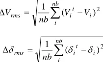
The algorithms are tested with a flat start and a convergence tolerance of 0.0001 per unit. In order to verify the accuracy of the resulting estimates, the following voltage magnitude and angle performance indices are calculated.
nb
i
i t i
rms V V
nb
V 1 ( )2 (11)
nb
i
i t i rms
nb
2 ) (
1
(12)
Table 1 Performance Comparison of Estimators
Test System Method ITER NET (ms) Vrms rms
IEEE-30
PM 5 612 1.6577e-6 7.7598e-7
RFDSE 8 80 5.1294e-6 1.4739e-6
WLS 3 210 5.0565e-6 1.4592e-6
WLAV 3 748 1.0783e-6 1.2390e-7
IEEE-57
PM 7 1455 1.1756e-7 9.0139e-7
RFDSE 11 220 1.5576e-6 2.2282e-7
WLS 4 495 1.9153e-6 2.4270e-7
WLAV 4 1960 1.1884e-7 2.5586e-7
69 node
PM 3 531 2.5204e-5 8.9910e-10
RFDSE 3 162 5.7463e-6 2.1435e-9
WLS 3 328 5.7230e-6 2.0798e-9
WLAV nc - - - - - - - - -
Table 1 compares the performance characteristics in terms of number of iterations (ITER), normalized execution time (NET), Vrms and rms. The PM reliably converges for all the test cases similar to WLS and RFDSE. The WLAV method alone diverges for the 69 node distribution system. The number of iterations of the PM is more than that of WLS and WLAV methods and less than that of RFDSE for 30 and 57 bus systems. However it takes the same number of iterations as that of WLS and RFDSE for 69-node distribution system. Analyzing the values of Vrms and rms, it is inferred that the proposed method performs well in terms of accuracy of the solution.
The computational burden can be studied precisely by analyzing the NET. The PM takes more execution time than that of WLS and RFDSE due to the use of time consuming LP. However, the PM takes lower execution time than that of WLAV due to the effect of decoupling and the use of constant sub-jacobian matrices.
PM are so small that they can be ignored due to its inherent property of rejecting bad measurements. Though the PM is slower than that of WLS method, it is robust in the sense that it is insensitive to r/ ratios like RFDSE x and has the capability of rejecting bad measurements like WLAV estimators and hence can be applied for real-time applications.
Table 2 Voltage Magnitude and Angle Indices with bad measurements for IEEE-30 bus system
NBD Vrms rms
WLS WLAV RFDSE PM WLS WLAV RFDSE PM
0 5.06e-6 1.08e-6 5.13e-6 1.68e-6 1.46e-6 1.24e-7 1.47e-6 7.76e-7 3 1.31e-3 1.04e-6 1.18e-3 1.68e-6 5.64e-5 1.25e-7 4.61e-5 7.72e-7 4 3.45e-3 1.11e-6 3.27e-3 1.68e-6 2.79e-4 1.23e-7 2.49e-4 7.78e-7 7 7.17e-3 3.18e-6 6.97e-3 3.57e-6 6.15e-4 3.08e-7 5.80e-4 2.76e-7 11 6.91e-3 2.74e-6 6.94e-3 3.49e-6 9.24e-4 2.36e-7 9.38e-4 1.13e-6 15 1.92e-2 5.11e-5 1.89e-2 5.67e-5 2.38e-3 3.43e-7 2.27e-3 2.18e-6 16 2.75e-2 4.15e-5 2.71e-2 4.15e-5 3.17e-3 2.36e-6 3.18e-3 2.35e-6 19 3.69e-2 5.10e-5 3.69e-2 5.98e-5 4.53e-3 2.28e-6 4.52e-3 4.14e-6 23 3.68e-2 5.69e-5 3.69e-2 5.61e-5 4.26e-3 4.31e-6 4.27e-3 4.53e-6 25 6.09e-2 1.43e-4 6.04e-2 1.42e-4 8.56e-3 1.23e-5 8.42e-3 1.26e-5 30 7.41e-2 3.11e-4 7.33e-2 3.21e-4 1.35e-2 1.95e-5 1.34e-2 2.20e-5
Table 3 Voltage Magnitude and Angle Indices with bad measurements for IEEE-57 bus system
NBD Vrms rms
WLS WLAV RFDSE PM WLS WLAV RFDSE PM
0 1.92e-6 1.18e-7 1.56e-6 1.18e-7 2.43e-7 2.56e-7 2.23e-7 9.01e-7 3 4.53e-4 1.25e-7 3.31e-4 1.16e-7 1.69e-5 2.48e-7 1.35e-5 1.51e-6 5 1.75e-4 3.16e-7 1.80e-4 1.29e-7 3.60e-5 2.90e-7 3.70e-5 1.44e-6 9 2.19e-3 3.15e-6 1.91e-3 8.69e-7 1.17e-4 4.44e-7 1.30e-4 9.73e-7 13 4.71e-3 2.77e-6 4.44e-3 1.61e-6 4.86e-4 1.08e-6 5.08e-4 7.50e-7 21 8.71e-3 4.17e-6 8.40e-3 4.68e-6 1.61e-3 1.36e-6 1.64e-3 5.90e-7 25 1.38e-2 2.65e-5 1.37e-2 2.69e-5 2.76e-3 4.62e-6 2.66e-3 1.55e-6 33 2.14e-2 2.46e-5 2.07e-2 2.59e-5 4.55e-3 4.10e-6 4.62e-3 6.57e-7 39 2.87e-2 2.31e-5 2.89e-2 2.58e-5 8.43e-3 8.41e-6 9.00e-3 1.95e-6 40 3.27e-2 2.31e-5 3.30e-2 2.58e-5 9.64e-3 8.41e-6 1.04e-2 1.95e-6 44 3.30e-2 2.05e-5 3.29e-2 2.20e-5 4.41e-3 6.22e-7 5.04e-3 5.82e-7
Table 4 Voltage Magnitude and Angle Indices with bad measurements for 69-node distribution system
NBD Vrms rms
WLS WLAV RFDSE PM WLS WLAV RFDSE PM
0 5.72e-6 2.90e-5 5.75e-6 2.52e-5 2.08e-9 7.41e-7 2.14e-9 8.99e-10 3 9.46e-5 2.44e-5 9.50e-5 2.52e-5 4.07e-8 3.69e-7 4.06e-8 8.99e-10 5 9.37e-5 3.41e-6 9.40e-5 2.81e-6 1.60e-8 3.16e-8 1.60e-8 5.15e-8 7 1.12e-3 1.73e-6 1.13e-3 3.29e-7 4.92e-7 1.38e-6 4.92e-7 3.76e-9 12 1.90e-3 4.12e-6 1.90e-3 3.18e-7 7.21e-7 2.56e-6 7.22e-7 1.03e-7 17 3.28e-3 1.30e-5 3.30e-3 2.18e-6 1.01e-6 1.84e-7 1.01e-6 2.16e-7 18 4.42e-3 2.02e-5 4.44e-3 4.82e-7 1.99e-6 1.88e-8 2.00e-6 4.17e-9 21 6.36e-3 1.28e-5 6.38e-3 1.23e-5 9.55e-7 1.36e-6 9.73e-7 1.36e-6 24 8.67e-3 1.76e-5 8.72e-3 1.58e-5 3.83e-6 1.46e-7 3.85e-6 1.97e-8 27 1.06e-2 7.40e-5 1.06e-2 7.36e-5 1.14e-6 6.83e-6 1.16e-6 6.99e-6
5. Conclusion
algorithm. It is tailor made to estimate the system state through the use of constant sub-jacobian matrices, which eliminate the computational burden and lower the execution time. The ability of the PM to reject bad measurements renders it to be more robust. The developed algorithm is found to be superior to the existing estimators in terms of accuracy, reliability and robustness; and is thus well suited for real-time applications. Acknowledgments
The authors gratefully acknowledge the authorities of Annamalai University for the facilities offered to carry out this work.
References
[1]. F. C. Schweppe and J. Wildes, “Power system static state estimation, part I: exact model”, IEEE Trans. on Power Appar. and Syst., Vol. PAS-89, pp. 120-125, 1970.
[2]. F. C. Schweppe and J. Wildes, “Power system static state estimation, part II: approximate model”, IEEE Trans. on Power Appar. and Syst., Vol. PAS-89, pp. 125-130, 1970.
[3]. R. E. Larson, W. F. Tinney and J. Peschon, “State estimation in power systems, part I: theory and feasibility”, IEEE Trans. on Power Appar. and Syst., Vol. PAS-89, No. 3, pp.345-352, 1970.
[4]. J. F. Dopazo, O. A. Klitin and L. S. Vanslyck, “State calculation of power systems from line flow measurements, Part II”, IEEE Trans. on Power Appar. and Syst., Vol. PAS-91, pp. 145-151, 1972.
[5]. S. A. Arafeh and R. Schinzinger, “Estimation algorithms for large scale power systems”, IEEE Trans. on Power Appar. and Syst., Vol. PAS-98, No. 6, pp. 1968-1977, 1979.
[6]. F. C. Schweppe and E. J. Handschin, “Static state estimation in electric power systems”, Proceedings of IEEE, Vol. 62, No. 7, pp. 972-982, 1974.
[7]. B.M. Zhang, S.Y. Wang, and N.D. Xiang, “A linear recursive bad data identification method with real time application to power system state estimation”, IEEE Trans. on Power Systems., Vol. 7, No. 3, pp.1378-1375, 1992.
[8]. H.A. Mangalvedekar, S.A. Khaparde, J.D. Parakkuth and S.D. Varwandkar, “Application of Parity Mismatches in detection of bad data for power system state estimation”, Electric Power Components and Systems, Vol. 27, No. 1, pp. 1-10, 1999.
[9]. M. R. Irving, R. C. Owen and M. J. H. Sterling, “Power system state estimation using linear programming”, Proceedings of IEE, Vol. 125, pp. 879-885, 1978.
[10].W. W. Kotiuga and M.Vidyasagar, “Bad data rejection properties of weighted least absolute techniques applied to static state estimation”, IEEE Trans. on Power Appar. and Syst., Vol. PAS-101, No.4, pp.844-853, 1982.
[11].Ali Abur, “A bad data identification method for linear programming for state estimation”, IEEE Trans. on Power Systems, Vol. 5, No. 3, pp. 894-901, 1990.
[12].H. P. Horisberger, J. C. Richard and C. Rossier, “A fast decoupled static state-estimator for electric power systems”, IEEE Trans. on Power Appar. and Syst., Vol. PAS-95, No.1, pp.208-215, 1976.
[13].N. D. Rao and S. C. Tripathy, “A variable step size decoupled state estimator”, IEEE Trans. on Power Appar. and Syst., Vol. PAS-98, No. 2, pp.436-443, 1979.
[14].J. J. Allemong, L. Radu and A. M. Sasson, “A fast and reliable state estimation algorithm for AEP’s new control center”, IEEE Trans. on Power Appar. and Syst., Vol. PAS-101, No. 4, pp. 933-944, 1982.
[15].W. M. Lin and J. H. Teng, “Distribution fast decoupled state estimation by measurement pairing”, IEE Proc. Gener. Transm. Distrib., Vol. 143, No. 1, pp. 43-48, 1996.
[16].W. M. Lin and J. H. Teng, “A new transmission fast-decoupled state estimation with equality constraints”, International Journal of Electrical Power and Energy Systems, Vol. 20, No. 7, pp. 489-493, 1998.
[17].L. Roy and T. A. Mohammed, “Fast super decoupled state estimator for power systems”, IEEE Trans. on Power Systems, Vol. 12, No. 4, pp. 1597-1603, 1997.
[18].F.F.Wu, “Theoretical study of the convergence of the fast decoupled load flow”, IEEE Trans on Power Apparatus and Systems, pp. 268-275, 1977.
[19].P.S.Nagendra Rao, K.S. Prakash Rao and J. Nantha, “A novel hybrid load flow method”, IEEE Trans on Power Apparatus and Systems, Vol. PAS-100, No. 1, pp. 203-308, 1981.
[20].Youman Deng, Ying He and Boming Zhang, “A branch estimation based state estimation method for radial distribution systems”, IEEE Trans. on Power Delivery, Vol. 17, No. 4, pp. 1057-1062, 2002.
[21].C. Madtharad, S. Premrudeepreechacharan, N. R. Watson, “Power system state estimation using singular value decomposition”, Electric Power Systems Research, Vol. 67, No. 2, pp. 99-107,2003.
[22].A. T. Saric and R. M. Ciric, “Integrated fuzzy state estimation and load flow analysis in distribution networks”, IEEE Trans. on Power Delivery, Vol. 18, No. 2, pp. 571-578, 2003.
[23].Du Zhengchun, Niu Zhenyong, Fang Wanliang, “Block QR decomposition based power system state estimation algorithm”, Electric Power Systems Research, Vol. 76, No. 1-3, pp.86-92, 2005.
[24].H.B Sun, B.M.Zhang, “Global state estimation for whole transmission for whole transmission and distribution networks”, Electric Power Systems Research, Vol. 74, No. 2, pp 187-195, 2005.
[25].M.K.Celik and A. Abur, “A robust WLAV state estimator using transformations”, IEEE Trans. on Power Systems, Vol. 7, No. 1, pp. 106-112, 1992.
[26].R. A. Jabr and B.C.Pal, “Iteratively reweighted least-square implementation of the WLAV state estimation method”, IEE Proc. Gener. Transm. Distrib., Vol. 151, No. 1, pp. 103-108, 2004.
[27].R. A. Jabr, “Power system state estimation using an iteratively reweighted least squares method for sequential L1-regression”,
International Journal of Electrical Power and Energy Systems, Vol. 28, No. 2, pp. 86-92, 2006.
[28].R. Neela and P. Aravindhababu, A new decoupling strategy for power system state estimation, Energy Conversion and Management, Vol. 50, No. 8, pp. 2047-51, 2009.
[29].P. Aravindhababu and R. Neela, “A reliable and fast decoupled WLS state estimation for power systems”, Electric Power Components and Systems, Vol. 36, No. 11, pp. 1200-1207, 2008.