https://doi.org/10.5194/cp-14-157-2018
© Author(s) 2018. This work is distributed under the Creative Commons Attribution 3.0 License.
Insights into Atlantic multidecadal variability using the Last
Millennium Reanalysis framework
Hansi K. A. Singh1, Gregory J. Hakim2, Robert Tardif2, Julien Emile-Geay3, and David C. Noone4 1Pacific Northwest National Laboratory, US Department of Energy, Richland, WA, USA
2Department of Atmospheric Sciences, University of Washington, Seattle, WA, USA
3Department of Earth Sciences, University of Southern California, Los Angeles, CA, USA
4College of Earth, Ocean, and Atmospheric Sciences, Corvallis, OR, USA
Correspondence:Hansi K. A. Singh ([email protected])
Received: 18 March 2017 – Discussion started: 15 May 2017
Revised: 24 October 2017 – Accepted: 29 November 2017 – Published: 9 February 2018
Abstract.The Last Millennium Reanalysis (LMR) employs a data assimilation approach to reconstruct climate fields from annually resolved proxy data over years 0–2000 CE. We use the LMR to examine Atlantic multidecadal variabil-ity (AMV) over the last 2 millennia and find several ro-bust thermodynamic features associated with a positive At-lantic Multidecadal Oscillation (AMO) index that reveal a dynamically consistent pattern of variability: the Atlantic and most continents warm; sea ice thins over the Arctic and re-treats over the Greenland, Iceland, and Norwegian seas; and equatorial precipitation shifts northward. The latter is con-sistent with anomalous southward energy transport mediated by the atmosphere. Net downward shortwave radiation in-creases at both the top of the atmosphere and the surface, indicating a decrease in planetary albedo, likely due to a de-crease in low clouds. Heat is absorbed by the climate system and the oceans warm. Wavelet analysis of the AMO time se-ries shows a reddening of the frequency spectrum on the 50-to 100-year timescale, but no evidence of a distinct multi-decadal or centennial spectral peak. This latter result is in-sensitive to both the choice of prior model and the calibra-tion dataset used in the data assimilacalibra-tion algorithm, suggest-ing that the lack of a distinct multidecadal spectral peak is a robust result.
1 Introduction
Studies of the observational and paleoproxy records pro-vide epro-vidence of multidecadal variability centered over the Atlantic. The Central England Temperature record, the longest observational temperature time series, suggests a 65-year timescale of variability over the last 350 65-years (Tung and Zhou, 2013). Evidence of multidecadal Atlantic vari-ability (with timescales anywhere between 20 and 80 years) has also been found in proxy tree ring records (Delworth and Mann, 2000; Gray et al., 2004), annually resolved ice cores (Chylek et al., 2011), and coral isotope records (Hetzinger et al., 2008). Lengthy proxy records extending over the last 8000 years also show multidecadal spectral power, though this power is not stationary over space or time (Knudsen et al., 2011).
Many studies have explored ocean–atmosphere interac-tions as driving factors for AMV, with changes in SSTs in the North Atlantic controlled by natural (unforced) fluctuations in the Atlantic meridional overturning circulation (AMOC) (see, e.g., Delworth et al., 1993; Polyakov et al., 2005; Zhang et al., 2007). Several dynamical studies using both ocean-only and fully coupled models have suggested that zonal and meridional oscillations in the AMOC on multidecadal timescales may drive changes in North Atlantic SSTs (for a description of the dynamical mechanism, see Raa and Di-jkstra, 2002; Dijkstra et al., 2006, 2008). While long-term observational records of the AMOC state are unavailable, observational evidence of sea surface height appears to sup-port the idea that North Atlantic SSTs covary with changes in sea surface height along the eastern seaboard of the United States, which is consistent with changes in the AMOC (Mc-Carthy et al., 2015).
Nevertheless, there remains disagreement regarding the role of AMOC changes in driving North Atlantic SST vari-ability over multidecadal timescales. (Tandon and Kushner, 2015) show that the relationship between AMV and the AMOC may not be stationary between the preindustrial and industrial periods: while AMOC fluctuations appeared to lead changes in North Atlantic SSTs over the preindustrial period in models, this lead–lag relationship reversed during the industrial era with strong anthropogenic forcing of the climate system (though there was substantial variations in the lead–lag relationship between models). Recently, (Clement et al., 2015) have shown that stochastic coupling between the atmosphere and oceanic mixed layer is sufficient to recover the AMV found in most climate models, calling into question the role of the oceanic MOC as a driver of the AMO. Indeed, only some state-of-the-art global climate models (GCMs) simulate multidecadal variability in Atlantic SSTs (Clement et al., 2015), while one older GCM has been shown to dis-play spurious multidecadal variability due to poor parameter-ization of ocean mixing processes (see Danabasoglu, 2008). (Hakkinen et al., 2011) suggest that changes in the strength of the North Atlantic subpolar and subtropical gyres may be more closely linked to the AMO than variations in the AMOC; such multidecadal shifts in the gyres alter
atmo-spheric blocking patterns which may, in turn, perturb SSTs over the entire Atlantic basin.
The role of aerosols and other forcings as external drivers of North Atlantic SST variability has also been debated. Aerosol release by volcanic eruptions has been suggested to act as an external driver of AMV in the preindustrial period (Ottera et al., 2010; Knudsen et al., 2014), contrary to other studies that suggest that AMV is internally driven by ocean– atmosphere interactions. Over the industrial period, the role of anthropogenic aerosols in driving AMV also remains an open question. (Booth et al., 2012) argue that aerosol di-rect and indidi-rect effects over the modern era (post-1850) have strongly impacted multidecadal SST variability over the North Atlantic, resulting in an evolution of North Atlantic SSTs that mimics an internally driven oscillation. This argu-ment, however, has been challenged by (Zhang et al., 2013), who suggest that the GCM used in (Booth et al., 2012) in-correctly modeled aerosol effects and show that improved representation of these effects reveals that 20th century sur-face temperature variations cannot be explained in full by changes in anthropogenic aerosol emissions. Nevertheless, more recent work by (Murphy et al., 2017) and (Bellucci et al., 2017) further challenges the premise that North At-lantic SST variability over the industrial period is unaffected by anthropogenic forcings.
Given major disagreements between climate models in AMO representation, it is clear that the study of AMO dy-namics would benefit from using observational data from the real Earth system. However, the detailed study of the AMO has been severely limited by the brevity of the in-strumental record, which is less than 2 centuries long. Fur-thermore, these observations are from a time period charac-terized by intense anthropogenic forcing of the climate sys-tem through greenhouse gases, aerosols, land use changes, ozone-depleting substances, and others. While the instru-mental record is short and likely biased towards a forced re-sponse, the proxy record does not suffer from this shortcom-ing. Indeed, annually resolved proxies for temperature from tree rings, corals, ice cores, and others exist at annual resolu-tion over the last several millennia. Although proxy records exist over much longer periods than observations, an objec-tive procedure for assimilating these proxies into coherent spatial fields remains an ongoing challenge.
in Steiger et al., 2014; Hakim et al., 2016), we will also note what additional information the assimilation of prox-ies yields beyond that found in this prior dataset. Finally, we will use the LMR to consider what, if any, robust timescales characterize the AMO over the last 2 millennia and how these timescales computed from the assimilation of the observa-tions compare to those found in previous studies.
The remainder of this paper is organized as follows. We describe the LMR proxy assimilation and climate field re-construction procedure, along with details of our regression and timescale analysis methodologies, in Sect. 2. In Sect. 3.1, we consider the AMO index over the last 2000 years, as in-ferred from the LMR, and in Sect. 3.2, we describe the ba-sic climate state that corresponds to a positive AMO index. We highlight the energetics associated with a positive AMO index in Sect. 3.3, particularly top-of-atmosphere and sur-face fluxes, the implied meridional energy transports, and flux imbalances. In Sect. 3.4, we consider timescales of the AMO using wavelet analysis. We conclude by discussing our findings, their implications, and caveats of our approach in Sect. 4.
2 Methods
The climate field reconstruction methodology used in the LMR is described in detail by (Steiger et al., 2014) and is val-idated for temperature reconstructions over the modern era (years 1850 to 2000 CE) in (Hakim et al., 2016).
The LMR uses a novel ensemble data assimilation proce-dure in which information from a prior expectation of the climate derived from a climate model is weighted against in-formation in proxy records. Weights are determined from the relative error in these two estimates of the climate, as defined by the update equation in the Kalman filter, which is optimal if the errors are Gaussian distributed. We proceed with an overview explanation of the Kalman update equation, before describing the solution method for this equation.
In brief, the data assimilation procedure updates the state of the prior,xp, to some new statexausing information from
the proxiesythat is weighted using a Kalman gain matrixK:
xa=xp+K(y−H(xp)). (1)
Here,His the observation model that converts the prior state to its proxy equivalent, H(xp). The innovation, y−H(xp), contains new information from the observations that is not al-ready present in the prior. The Kalman gain matrixK, which weights the innovation and maps from proxy space to physi-cal space, is
K=BHT(HBHT +R)−1, (2)
whereBis the error covariance matrix for the prior data,His the linearization of the observation modelHabout the prior mean, and Ris the error covariance matrix for the proxies (described further below). The numerator of matrixK,BHT,
is the covariance expectation between the prior and the prior estimated observations and acts to spread information from proxy locales into the physical space.
The solution to Eqs. (1) and (2) is fully described in (Steiger et al., 2014) and (Hakim et al., 2016), and a sum-mary of the essential elements follows. First, we describe our method for estimating the proxies from the prior data (i.e.,H) and the associated errors (i.e.,R). Second, we describe our method for creating the prior and the associated errors (i.e.,
xpandB) using an ensemble sampling technique. This en-semble technique relates directly to the solution method for Eqs. (1) and (2).
The observation modelH, a forward model that maps from physical space to the proxy space, is constructed using a cali-bration dataset and assumes a linear relationship between the proxy state and temperature over the calibration period:
y=β0+β1T0+, (3)
whereT0 is the annual mean 2 m air temperature anomaly from the calibration dataset, β0 is the intercept, β1 is the slope, andis a Gaussian random variable with zero mean and a variance ofσ2. The calibration temperature T0 for a given proxy record is chosen from the grid point closest to the proxy location at concurrent time periods, and parame-tersβ0,β1, andσ are computed using a linear least-squares fit against the NOAA Merged Land–Ocean Surface Temper-ature Analysis (MLOST; Smith et al., 2008) during the time period 1900–2000. The diagonal elements ofR, the error co-variance matrix for the proxies, are the co-variance of the re-gression residuals,σ2. In principle, other sources of error contribute toR, such as instrumental (laboratory) error and representativeness error (the climate model grid cell resolves spatial averages rather than the points that are observed), but the errors in Eq. (3) are large by comparison and so we ap-proximateRaccordingly.
year in the reconstruction. The mean value of this sample serves asxpin Eq. (1).
We use an ensemble square-root solution method to Eqs. (1) and (2), including serial observation processing (Whitaker and Hamill, 2002), so that proxies are assimi-lated one at a time for each year of the reconstruction. In this approach, the matrix inverse in Eq. (2) becomes a triv-ial scalar inverse, and the covariance matrix B, which can be enormous, is never explicitly formed; rather, only the ensemble-estimated covariance between the proxy and the reconstructed field at each point is needed (see Steiger et al., 2014, for further details). Proxy estimates H(xp) are com-puted in advance and updated each year along with the re-constructed fields with the assimilation of each proxy.
Using this method, we reconstruct annual mean fields be-tween 0 and 2000 CE. The proxies used are a total of 465 time series from the PAGES2K dataset (Consortium, 2013; Hakim et al., 2016), which includes lake sediment calcium to phosphorus ratios, ice core water isotopes (both oxygen and hydrogen), coral oxygen isotopes, tree rings (width and den-sity), and speleothem water isotopes. As described in (Hakim et al., 2016), the LMR reconstructions of temperature and 500 hPa geopotential height have been validated over the in-strumental period. Moreover, the results have also been val-idated against independent proxies (not assimilated) before and during the instrumental period and to ensure that the er-ror in the ensemble mean is statistically equivalent to the pre-dicted error in the ensemble variance as expected from the-ory. Though the reanalysis results obtained when using dif-ferent prior and observation–model calibration datasets are quantitatively distinct (see Fig. 12 in Hakim et al., 2016), they all yield qualitatively similar results. Therefore, much of the ensuing analysis, apart from the calculation of timescales (see below), is performed using this single reanalysis, here-after referred to as MLOST-CCSM4.
We note that because the prior is the same for every year, all temporal variability is determined by the proxies. As a re-sult, the weighting in Eq. (1) involves a temporally invariant prior and temporally variable proxies so that, for any given proxy, reduced temporal variability may be expected. How-ever, since the time series at any point in the reconstruction depends on the prior and many proxies all having different er-rors, the variability at a proxy location may in fact be larger or smaller than that of a given proxy at that point.
Following (Clement et al., 2015) and others, we quantify AMV using the AMO index, which is computed annually as the average of the area-weighted SSTs from 60◦N to the
Equator and 80◦W to the prime meridian. Links between
cli-mate variables and the AMO are defined by regression onto the AMO index and computing the value of the variable at two SDs of the AMO index. In order to isolate multidecadal (and longer) timescale variability, both the AMO index and variable fields are filtered using a 20-year low-pass Lanc-zos filter with 31 filter weights prior to computing the re-gressions (unless otherwise noted; see Duchon, 1979, for a
full description of the Lanczos filter). The AMO index and climate variable fields are detrended before regression. Re-gression results from the LMR are computed for three time periods to highlight potential nonstationarity in the AMO: years 0 to 1850 (the preindustrial era), 1200 to 1850 (the part of the preindustrial era when proxy coverage is substantial), and 1850 to 2000 (the industrial era). These results are com-pared to similar results from the CCSM4 prior.
AMO index timescale analysis was performed with wavelets using the methodology described by (Torrence and Compo, 1998). The Paul wavelet is used with a scale spac-ing of 0.25 and a total of 52 scales spannspac-ing 2 to 1000 years. Significance is computed at p <0.05 using a one-step au-toregression (AR(1); i.e., red noise) process as the null hy-pothesis; significance results were found to be insensitive to the choice of the mother wavelet. Wavelet analysis was per-formed on six different AMO index reconstructions using two different priors and three different calibration datasets (see Table 1).
3 Results
3.1 The AMO index in the LMR
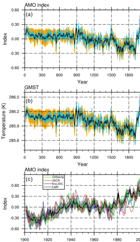
Over the last 2000 years, the AMO index reconstructed from the LMR resembles the global mean surface temper-ature (GMST) time series (Fig. 1a and b;r=0.97 at lag 0). Like the GMST, the AMO has the least variability over the first 1000 years of the reanalysis, possibly due to the lack of globally distributed proxy records over this early period of the reanalysis. Over the latter portion of the reanalysis (year 900 CE forward), a cooling trend is evident in both the AMO and GMST, which is punctuated by a warmer period centered at year 1500 CE. A warming trend is evident in both the AMO and GMST time series following year 1900 CE.
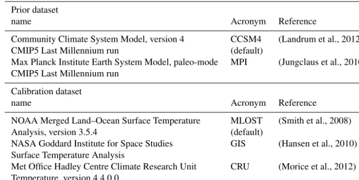
Table 1.Prior and calibration datasets used in the LMR reconstruction. The default datasets are used for all analyses, while additional datasets are only used in the wavelet timescale analyses.
Prior dataset
name Acronym Reference
Community Climate System Model, version 4 CCSM4 (Landrum et al., 2012)
CMIP5 Last Millennium run (default)
Max Planck Institute Earth System Model, paleo-mode MPI (Jungclaus et al., 2010) CMIP5 Last Millennium run
Calibration dataset
name Acronym Reference
NOAA Merged Land–Ocean Surface Temperature MLOST (Smith et al., 2008)
Analysis, version 3.5.4 (default)
NASA Goddard Institute for Space Studies GIS (Hansen et al., 2010) Surface Temperature Analysis
Met Office Hadley Centre Climate Research Unit CRU (Morice et al., 2012) Temperature, version 4.4.0.0
3.2 Thermodynamics of the AMO in the LMR
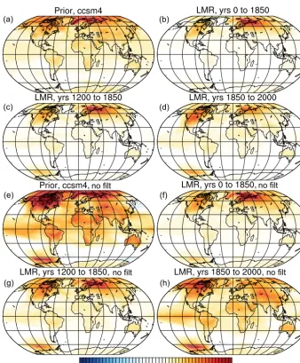
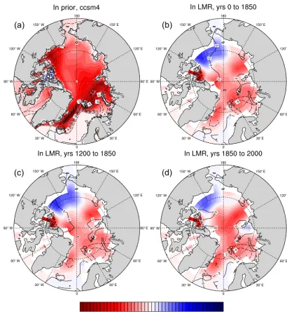
Globally, the temperature field associated with a positive AMO index is characterized by warming over the continents and especially strong warming over the far northern reaches of the Atlantic and Arctic (Fig. 2). Warming is greater over the Northern Hemisphere (NH) than the Southern Hemi-sphere (SH) over all time periods, and the magnitude of warming is strongest over all regions in the CCSM4 prior compared to that in the LMR. Over both the CCSM4 prior and the LMR, there is warming over the Arctic, though the location of maximum warming is different: in the CCSM4 prior, warming is greatest over the Greenland, Iceland, and Norwegian (GIN) seas, while warming is greatest in the LMR over the Barents Sea. In the LMR, variability is rela-tively stationary over all time periods (r=0.92 between the regression over years 0 to 1850 andr=0.73 over years 1200 to 1850 and years 1850 to 2000), though differences in warm-ing over the high northern latitudes are apparent; in the prein-dustrial period (pre-1850), warming over northern Eurasia is most prominent, while warming over boreal North America and central Asia dominates in the industrial period.
Comparison of the 20-year low-pass-filtered regression of the AMO index on temperature (Fig. 2a to d) with the un-filtered regression (Fig. 2e to h) reveals that the temperature response associated with the AMO is stronger on the shorter timescales that dominate the unfiltered regression.
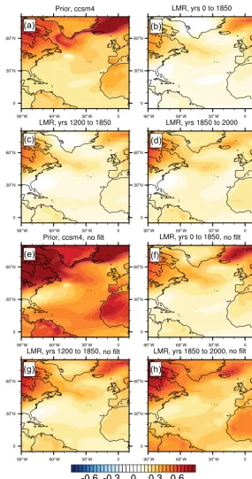
Over all time periods in the LMR (years 0 to 1850, years 1200 to 1850, and years 1850 to 2000), warming is not uniform over the North Atlantic basin: maxima in warm-ing are evident at 50 and 5◦N (Fig. 3a to d). Over shorter timescales than those explored in the remainder of this study, however, the two-lobed pattern becomes a horseshoe with the tropical and midlatitude warming maxima linked by warm-ing over the eastern Atlantic (compare Fig. 3a–d to Fig. 3e–
h). This distinct horseshoe pattern of warming over the mid-latitudes and tropics that characterizes North Atlantic SST variability on shorter timescales has been noted by others and is the leading mode of variability found with empirical or-thogonal functional decomposition analysis over this region (see, e.g., Hartmann, 1994). Because our focus is on longer-timescale variability, we will utilize 20-year low-pass filter-ing for the rest of our analysis (except for time series analysis of the AMO index; Sect. 3.4).
During the positive phase of the AMO, the LMR shows that warming over the high-latitude North Atlantic is linked to the retreat of sea ice from the GIN and Barents seas (Fig. 4, contours), with strong spatial agreement between the LMR over all time periods (r=0.89 between the regression over years 0 to 1850 andr=0.69 over years 1200 to 1850 and years 1850 to 2000). In contrast, the CCSM4 prior shows a much more sharply defined spatial pattern of sea ice retreat than the LMR, though the general regions of retreat are the same. Sea ice also thins over much of the Arctic (Fig. 4, col-ors) in both the LMR and CCSM4 prior; in the CCSM4, sea ice thins over the entire Arctic, while in the LMR, there is a small region of sea ice thickening centered about the Beau-fort Sea. This thickening of ice in the BeauBeau-fort sea is linked to a low pressure center over the Arctic in the LMR, which is not present in the CCSM4 prior (or in other reanalyses of the instrumental period). Sea ice retreat coincident with the pos-itive phase of the AMO has also been shown in model-based studies (see, e.g., Miles et al., 2014). Such retreat and thin-ning of sea ice is also consistent with increased ocean heat transport into the North Atlantic, possibly due to strength-ening of the AMOC during the positive phase of the AMO (considered further in Sect. 3.3).
Equa-( )
( )
( )
Figure 1.(a)Atlantic Multidecadal Oscillation (AMO) index time series and(b)global mean surface temperature (GMST) time se-ries computed from the LMR over the last 2000 years, with the yearly time series (light blue, dotted) and 20-year low-pass time series (black; 95 % confidence interval shown in orange).(c)AMO index over the last 100 years (bottom) as computed from the LMR (black; 95 % confidence interval shown in grey), the 20th Century Reanalysis (20CR, red), the ERA-20C reanalysis (Era-20C, blue), and the NASA GIStemp reanalysis (GIStemp).
tor over all basins (Fig. 5). Surprisingly, the magnitude of these changes is larger in the LMR (years 1200 to 1850 and years 1850 to 2000) than in the CCSM4 prior, though tem-perature increases associated with the AMO are largest in the latter (recall Fig. 2). On the other hand, the magnitude of these changes is very small over years 0 to 1850 CE in the LMR, possibly due to poor proxy coverage during the earlier part of this period. Most changes in precipitation are colo-cated in the CCSM4 prior and the LMR (r=0.51,0.45,0.55 between the CCSM4 and the LMR over years 0 to 1850, 1200
to 1850, and 1850 to 2000, respectively), though the LMR predicts stronger AMO-linked drying over the maritime con-tinent than found in the CCSM4 prior. In general, the mag-nitude of the increase in precipitation is greatest in the NH, and a northward shift in the equatorial precipitation maxi-mum (the Intertropical Convergence Zone, i.e., the ITCZ) is particularly evident over the Atlantic basin (see also Knight et al., 2006). We also note that the double ITCZ apparent in the CCSM4 prior is consolidated into a single precipitation maximum in the LMR.
3.3 Energetics
The energetics associated with a positive AMO index differ significantly between the LMR and the CCSM4 prior. While surface and TOA fluxes and their imbalances are qualitatively similar between the LMR and the CCSM4 prior, we find that the energy transports implied by these fluxes differ between the LMR and CCSM4 prior. Overall, the energetics and im-plied dynamics in both the LMR and CCSM4 prior are con-sistent with most findings from previous studies (see Knight et al., 2006), though there are some discrepancies. We de-scribe these findings in detail below.
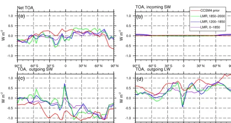
In the LMR, a positive AMO index is linked to net top-of-atmosphere (TOA) radiative flux (positive upward) anoma-lies that are negative in the NH and positive in the SH over all time periods (Fig. 6a). While the anomaly in the TOA in-coming shortwave (SW) flux is nearly zero (Fig. 6b), large compensating changes in the outgoing SW flux and outgo-ing longwave (LW) flux mostly determine the net TOA ra-diative flux (Fig. 6c and d, respectively). The outgoing SW flux anomaly is negative nearly everywhere (i.e., the outgo-ing SW flux decreases), with the LMR showoutgo-ing the strongest anomalies north of the Equator. These anomalies are consis-tent with either an increase in atmospheric SW absorption by water vapor in the warmer hemisphere or a decrease in re-flected SW due to fewer clouds in the warmer hemisphere. The outgoing LW flux increases nearly globally, commen-surate with increased temperatures at the effective radiating level associated with warming during the positive phase of the AMO. This increase in outgoing LW radiation dominates in the SH, while the decrease in outgoing SW radiation domi-nates in the NH, implying a net southward meridional energy transport in the LMR (see Fig. 8a and accompanying text). At the Equator, there is an increase in the outgoing SW ra-diation, which is balanced by a decrease in the outgoing LW radiation; both are consistent with greater cloudiness in the deep tropics and strengthening of the equatorial precipitation noted earlier (Fig. 5).
im-(a) (b)
(c) (d)
(e) (f)
(g) (h)
no filt no filt
no filt no filt
Figure 2.Low-pass-filtered regression of the AMO index on surface temperature (in K) in(a)the CCSM4 prior,(b)the LMR from years 0 to 1850,(c)the LMR from years 1200 to 1850, and(d)the LMR from years 1850 to 2000. Panels(e)through(h)are similar to(a)through
(d), but show the unfiltered regression.
plied meridional total energy transport in the CCSM4 prior is polewards in both hemispheres.
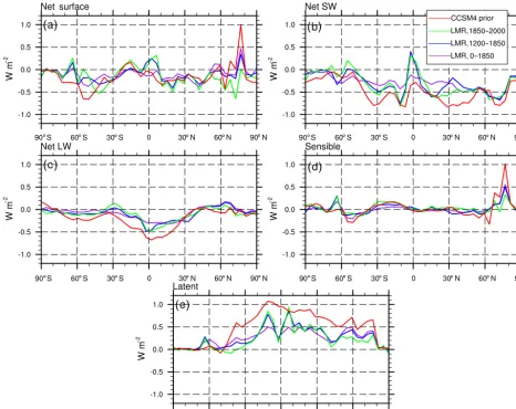
At the surface, both the LMR and the CCSM4 prior have net fluxes associated with a positive AMO index that are downwards in the tropics, upwards in the subtropics and mid-latitudes, and downwards in the NH high latitudes (Fig. 7a). This pattern is most pronounced in the CCSM4 prior, but is also evident over all time periods in the LMR. Globally, we find that this spatial pattern results from decreases in both the net (upward) surface SW radiation (i.e., an increase in SW coming down at the surface; Fig. 7b) and the net (up-ward) surface LW radiation (i.e., an increase in the LW com-ing down at the surface; Fig. 7c); these increased surface SW and LW radiative fluxes are mostly balanced by an increase in the surface latent heat flux (Fig. 7e), which renders the
net surface flux small over most latitudes. At the Equator, an increase in the net (upward) surface SW radiation and a de-crease in the net (upward) surface LW radiation is consistent with greater cloud cover. Sensible heat flux anomalies at the surface are small everywhere (Fig. 7d).
(a) (b)
(c) (d)
(e) (f)
(g) (h)
no filt no filt
no filt no filt
°
° °
°
°
° °
°
°
° °
°
°
° °
°
° ° °
° ° °
° ° °
° ° °
° ° °
° ° °
° ° °
° ° °
Figure 3.As in Fig. 2 over the North Atlantic basin.
As alluded to earlier, differences in the net TOA radiative fluxes between the LMR and the CCSM4 prior imply very different total energy transport anomalies. The total implied meridional energy transport, TET, at latitudeφ0can be com-puted using the zonally averaged net TOA fluxes RTOA(φ)
as
TET(φ0)=rearth2 2π Z
0
φ0
Z
0
Figure 4.As for Fig. 2 panels(a)to(d), but for the low-pass-filtered regression of the AMO index on sea ice thickness (colors, in millimeters) and on sea ice concentration (contours, %).
where φ and θ are the latitude and longitude coordinates, respectively, rearth is the radius of Earth, and Rstorage(φ) is the heat storage tendency of the climate system at latitude φ(Peixoto and Oort, 1992). We find that the TET is anoma-lously southward north of 20◦S and northward south of 20◦S for the LMR over later time periods (1200 to 1850 and 1850 to 2000) and is particularly large between 10◦S and 20◦N (Fig. 8a). In the CCSM4 prior, on the other hand, the TET is anomalously southward south of 10◦N and anomalously northward north of 10◦N.
The atmospheric energy transport, AET, at latitude φ0 is computed using the difference betweenRTOA(φ) and net
sur-face fluxRSfc(φ) as
AET(φ0)=rearth2 2π Z
0
φ0 Z
0
(RTOA(φ)−RSfc(φ)) cos(φ)dφdθ. (5)
Figure 5.As for Fig. 2 panels(a)to(d), but for the low-pass-filtered regression of the AMO index on precipitation (in mm day−1).
( ) ( )
( ) ( )
° ° ° ° ° ° ° ° ° ° ° °
° ° ° ° ° °
° ° ° ° ° °
Figure 6.Low-pass-filtered regression of the AMO index on top-of-atmosphere (TOA) energy fluxes (in W m−2) in the LMR (from years 0 to 1850, 1200 to 1850, and 1850 to 2000) and the CCSM4 prior:(a)net (incoming) flux,(b)incoming shortwave (SW) flux,(c)outgoing SW flux, and(d)outgoing longwave (LW) flux.
(recall Fig. 5). The increase in southward cross-equatorial energy transport is also consistent with an increase in the interhemispheric temperature difference associated with the AMO that preferentially warms the NH over the SH (recall Fig. 2; also see Friedman et al., 2013), which arises from a strengthening of the Hadley circulation in the cooler hemi-sphere. On the other hand, the increase seen in the CCSM4
prior occurs most prominently in the midlatitudes, suggest-ing a strengthensuggest-ing of poleward energy transport by midlati-tude eddies in the SH rather than an adjustment of the tropical circulation.
The oceanic energy transport OET(φ0) is computed as a residual from the TET and AET:
° ° ° ° ° ° ° ° ° ° ° °
° ° ° ° ° ° ° ° ° ° ° °
° ° ° ° ° °
( ) ( )
( ) ( )
( )
Figure 7.Low-pass-filtered regression of the AMO index on surface energy fluxes (in W m−2) in the LMR (from years 0 to 1850, 1200 to 1850, and 1850 to 2000) and the CCSM4 prior:(a)net (downward) surface flux,(b)net (upward) SW flux,(c)net (upward) LW flux,(d)
sensible heat flux, and(e)latent heat flux.
From Fig. 8c, it is clear that, aside from the subtropical SH, the LMR and CCSM4 prior differ significantly in anoma-lous OET associated with the positive phase of the AMO. In the LMR (over 1200 to 1850 and 1850 to 2000), energy transport by the ocean is anomalously southward in the NH and northward in the SH, with a significant southward cross-equatorial component; much of the anomalous transport is confined to the subtropics. These anomalies are larger over the 1850–2000 time period and are consistent with a decrease in oceanic energy transport by the wind-driven subtropical gyres and subtropical cells when the AMO is in its posi-tive phase. A large southward cross-equatorial component to the OET anomaly suggests a decrease in northward cross-equatorial energy transport by the AMOC. In the CCSM4 prior, on the other hand, the OET response is anomalously positive at all latitudes, suggesting that an increase in north-ward energy transport by the AMOC corresponds to a posi-tive AMO index.
In both the LMR and CCSM4 prior, we find that the av-erage net TOA flux over the last 2000 years is positive, indi-cating that energy is being removed from the Earth system; when the AMO index is positive, however, the net TOA flux decreases such that energy is being anomalously added to the Earth system relative to the mean state (Table 2). The extent to which this occurs is similar between the CCSM4 prior and the LMR over all time periods, suggesting that this aspect of the AMO has been stationary over the last 2000 years.
posi-Table 2.Net top-of-atmosphere (TOA) flux imbalances in the LMR (from years 0–1850, 1200–1850, and 1850–2000) and the CCSM4 prior shown for the global mean and regressed on the AMO index. Fluxes out of the Earth system (i.e., upward) are positive.
Net TOA imbalance (W m−2) Global mean Regressed on the AMO index
LMR, 0–1850 0.46 0.01
LMR, 1200–1850 0.31 −0.01
LMR, 1850–2000 0.37 0.01
CCSM4 prior 0.61 0.19
( )
( ) ( )
° ° °
° ° °
° ° °
° ° °
° ° °
° ° °
Figure 8.Low-pass-filtered regression of the AMO index on energy transport (in PW) in the LMR:(a)total energy transport,(b) atmo-spheric energy transport, and (c)oceanic energy transport for the LMR from years 0 to 1850 (purple lines), the LMR from years 1200 to 1850 (blue lines), the LMR from years 1850 to 2000 (green lines), and CCSM4 prior (red).
tive AMO index, which also decreases relative to the mean. The results from the CCSM4, however, are more energeti-cally consistent in the magnitude of the energy uptake by the climate system when the AMO is in its positive phase (0.19 and 0.18 W m−2for the TOA and surface flux imbalances, re-spectively) compared to the LMR (e.g., 0.01 and 0.13 W m−2
for the TOA and surface flux imbalances, respectively, in the LMR over the years 0 to 1850 CE).
3.4 Timescales of variability
We now consider what timescales characterize the AMO in-dex. (Tung and Zhou, 2013) show a distinct 50- to 80-year peak in the Central England Temperature record (HadCET; see Parker et al., 1992) and suggest that this variability may be related to coherent variability in North Atlantic SSTs. Other studies have synthesized proxy records from the North Atlantic basin over the last 500 years to infer the existence of such a multidecadal oscillation over the last millennium (see Delworth and Mann, 2000; Gray et al., 2004). Furthermore, (Knudsen et al., 2011) suggest that multidecadal variability that is nonstationary and possibly linked to North Atlantic SSTs is evident in global ice core and sedimentary records over a span of the last 8000 years.
Motivated by previous research, we now analyze what timescales are evident in the LMR reconstruction of North Atlantic SSTs. The LMR uses records from proxies over the last 2 millennia weighted heterogeneously relative to the prior and includes the proxy data used by Delworth and Mann (2000), Gray et al. (2004), and others; these records are processed here using the data assimilation algorithm described herein (see Sect. 2; Hakim et al., 2016). If the timescales present in individual proxy record time series are indicative of variability over the large-scale North Atlantic in general, these timescales should also be present in the recon-structed AMO index.
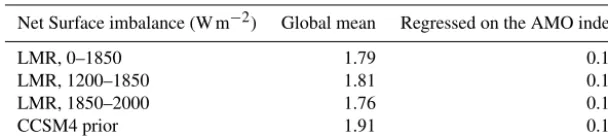
Table 3.Net surface flux imbalances in the LMR (from years 0–1850, 1200–1850, and 1850–2000) and the CCSM4 prior shown for the global mean and regressed on the AMO index. Fluxes out of the surface (i.e., upward) are positive.
Net Surface imbalance (W m−2) Global mean Regressed on the AMO index
LMR, 0–1850 1.79 0.13
LMR, 1200–1850 1.81 0.12
LMR, 1850–2000 1.76 0.14
CCSM4 prior 1.91 0.18
of the reconstructions reveal an event at year 500; this may reflect either a lack of proxy records over this period or non-stationarity in the climate system over the preindustrial pe-riod.
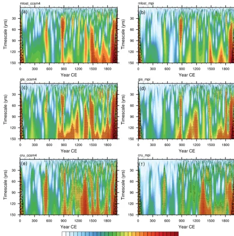
We assess the significance of variability on these different timescales using the global wavelet power spectrum, which is an average of the coincident wavelet power on each timescale over the entire record. These global power spectra, shown in Fig. 10a, suggest that there is no distinct multidecadal spec-tral peak in the AMO index. Many of the reconstructions suggest reddening of the spectrum near the 50- to 60-year timescale, particularly those reconstructions using the GIS and MLOST calibration datasets, though none of these are statistically significant atp <0.05. Furthermore, reconstruc-tions using the CRU calibration dataset show that longer-timescale (≥90 year) variability cannot be explained by a simple AR(1) process. However, our results appear to rule out the presence of distinct multidecadal oscillations in North Atlantic SSTs over the last 2 millennia. We find that this re-sult is insensitive to the wavelet type and is not affected if a shorter time period is used for the analysis (e.g., years 1200 to 2000 CE). Furthermore, we find that the global power spectrum is very quantitatively similar when the same anal-ysis is performed using a fixed-proxy network for the recon-struction (i.e., one in which all proxy records are continuous for the entire time period of the analysis), further suggesting that these results are insensitive to the choice of proxy net-work used. In addition, multitaper spectra (Thomson, 1982) confirm that none of our AMO reconstructions exhibit any spectral power on multidecadal timescales above that ex-pected from red noise (see the Supplement), which is con-sistent with results gleaned from the global wavelet power spectrum (Fig. 10a).
While we do not find a statistically significant multi-decadal spectral peak in the AMO index, we do find a sig-nificant 3- to 4-year spectral peak (Fig. 10b). We suggest that this peak may be a result of teleconnections with the tropical Pacific and El Niño–Southern Oscillation (ENSO) variability therein, which has a similar timescale (see, e.g., Dong et al., 2006). We reserve study of connections between tropical Pa-cific and Atlantic variability for future work.
3.5 Limitations of LMR investigation of the AMO and other variability
While we have been able to show that the LMR captures ther-modynamic aspects of the AMO, there are factors that limit its utility in investigating the dynamics of the AMO. While proxy records synthesize information about temperature and precipitation, their utility for reconstructing fields that are relatively invariant to temperature remains uncertain. We find that dynamic spatial fields like surface pressure and winds are not well reconstructed by the LMR (not shown); there-fore, we have not included such reconstructions in this analy-sis. The limitations of paleoclimate reanalyses using proxies that record primarily thermodynamic variables, rather than dynamic ones, remains an open question that will be consid-ered in future work.
4 Discussion
We have considered the thermodynamics of the AMO over the last 2000 years using the LMR, a paleoclimate reanaly-sis method that objectively assimilates information from pa-leoclimate records. Several aspects of our findings regard-ing the AMO agree with previous model-based and obser-vational studies of North Atlantic SST evolution. We find that a positive AMO index coincides with warmer conti-nents, a two-lobed pattern of warming over the Atlantic, and a warmer Arctic (Kushnir, 1994; Delworth and Mann, 2000; Chylek et al., 2009). In the Arctic, sea ice retreats from the Greenland, Iceland, and Nordic seas and thins over much of the Arctic Ocean (Miles et al., 2014). Globally, precipita-tion increases and the ITCZ strengthens and shifts northward (Knight et al., 2006).
Figure 9.Wavelet analysis of AMO time series from six different LMR reconstructions (in units of variance of the AMO index,K2):
(a)MLOST-CCSM4,(b)MLOST-MPI,(c)GIStemp-CCSM4,(d)GIStemp-MPI,(e)CRU-CCSM4, and(f)CRU-MPI. All analyses are performed using the Paul wavelet. Stippled areas are statistically significant atp <0.05, and the hatched region demarcates the cone of influence.
by the oceans. TOA and surface flux anomalies are consis-tent with an increase in atmospheric specific humidity and a decrease in low (reflective) clouds.
Our study of the AMO using the LMR demonstrates that climate field reconstruction methods, which assimilate infor-mation from the proxy record, can provide valuable informa-tion on climate variability in the Earth system. While cor-relations between North Atlantic SSTs and various thermo-dynamic fields (temperature, precipitation, and sea ice) are
character-Figure 10. Global wavelet spectra of reconstructions shown in Fig. 9(a)for timescales between 0 and 200 years and(b)zoomed in to show timescales between 2 and 10 years. Timescales that are sta-tistically significant over the red noise background (atp <0.05) are shown as solid lines, while timescales that are not statistically sig-nificant are shown as dotted lines. In units of variance of the AMO index,K2.
ize the AMO. Since there is little agreement between various GCMs regarding the dominant timescales that characterize the AMO (see Clement et al., 2015), LMR reconstruction of the AMO index is invaluable. Our results suggest that the proxy observations over the last 2000 years, when objectively assimilated, do not exhibit a multidecadal timescale.
The lack of a distinct multidecadal spectral peak in the LMR reconstruction of the AMO is in contrast to other stud-ies that have found such variability in individual observa-tional records (see, e.g., Tung and Zhou, 2013) or limited collections of proxies (see, e.g., Delworth and Mann, 2000; Gray et al., 2004). We point out that such a significant spec-tral peak in an individual record or collection of records does not necessarily translate into a coherent mode of basin-scale multidecadal variability. While certain records may display oscillations, a basin-scale oscillation requires both spatial co-herence and matching timescales in these records over cer-tain regions. The objective assimilation procedure used in
the LMR climate field reconstruction utilizes the information provided by the proxy records investigated in these previous studies; the results of this objective assimilation suggest that there is no distinct multidecadal or centennial spectral peak in the AMO index, though there is reddening of the spec-tra. These results support the null hypothesis presented by (Clement et al., 2015) and suggest that there may be little need to consider longer-timescale processes when studying the mechanism of the AMO over the late Holocene, particu-larly the preindustrial period.
In our reconstructions, multidecadal spectral power is evident only over the latter portion of the LMR, year 1500 CE forward, and is particularly pronounced fol-lowing year 1900 CE. While there has been much hypothe-sized regarding these oscillations in the instrumental record and whether they are a result of internal climate variability or a result of external forcing (see, e.g., Booth et al., 2012; Zhang et al., 2013; Murphy et al., 2017; Bellucci et al., 2017, and others), we point out two important characteristics of the instrumental period that render it a poor era for study-ing multidecadal variability in the climate system. First, the instrumental record is very short; as a result, there is very little that can be said about multidecadal timescale variabil-ity over this time period that carries any statistical weight (see, e.g., Wunsch, 1999; Vincze and Janosi, 2011). Second, the instrumental period is one in which the climate system has been strongly anthropogenically forced, suggesting that any variability observed over this period may differ signif-icantly from variability from the preindustrial era when an-thropogenic forcing was much smaller. Indeed, (Tandon and Kushner, 2015) show that in models, the lead–lag relation-ships between North Atlantic SSTs and the AMOC are very different between the preindustrial and modern periods, sug-gesting a shift in the mechanism underlying AMV between these two time periods. Both of these limitations suggest that caution must be exercised in extrapolating characteristics of multidecadal variability in the Earth system from the instru-mental record.
We also point out that our objective data assimilation ap-proach cannot completely rule out a distinct multidecadal spectral peak in North Atlantic SSTs. While we have shown that objective data assimilation of the proxy record to recon-struct the surface temperature field over the last 2 millen-nia does not yield any evidence of multidecadal variability, it is likely that further improvements in the proxy network, the proxy system models, or the data assimilation procedure will improve the reconstruction in such a way as to modify our current conclusions. From this study, however, we can say that the surface temperatures reconstructed over the last 2000 years, which are obtained from assimilating the exist-ing network of proxies usexist-ing today’s state-of-the-art meth-ods, do not provide compelling evidence for multidecadal oscillations over the North Atlantic.
assimilation approach itself is Gaussian, which may limit its utility in regimes very different from that of the base climate state. Second, LMR reconstructions depend on the climate models, proxies, and observation models that are used to cre-ate them. These components, in turn, are being continually tuned and refined. Third, it is unknown what effects the limi-tations in the size and distribution of the proxy network have on the reconstruction made possible by the LMR. In partic-ular, we note that the more limited network from the early portion of the instrumental record (pre-1200 CE) may affect the reconstruction and its variability. Further study will be required to assess sensitivity to the sparsity of the proxy net-work. Finally, we note that there are other ways to improve paleoclimate reanalyses using proxy records, including the incorporation of linear inverse modeling into the reconstruc-tion methodology to achieve online data assimilareconstruc-tion (see Perkins and Hakim, 2016). In the future, such refinement of reconstruction methods will help to further the study of the Earth system over its long and varied climatic history.
Code availability. The data assimilation software for the LMR project will be publicly released on BitBucket and GitHub at the end of the project in 2018.
Data availability. Datasets used in this study are pub-licly available on the Zenodo data archiving service: https://doi.org/10.5281/zenodo.1162342 (Singh, 2018).
Supplement. The supplement related to this article is available online at: https://doi.org/10.5194/cp-14-157-2018-supplement.
Competing interests. The authors declare that they have no con-flict of interest.
Acknowledgements. Hansi K. A. Singh thanks Andre Perkins for informative discussions and technical help. All authors ac-knowledge funding support from the following sponsors to the University of Washington: the National Science Foundation (awards AGS-1304263 and AGS-1602223) and the National Oceanic and Atmospheric Administration (award NA14OAR4310176). All authors also acknowledge the World Climate Research Program’s Working Group on Coupled Modeling, which is responsible for CMIP, and thank the climate modeling groups (CCSM4 and MPI, listed in Table 1) for producing and making available their model output. For CMIP the US Department of Energy’s Program for Climate Model Diagnosis and Intercomparison provides coordinat-ing support and led the development of software infrastructure in partnership with the Global Organization for Earth System Science Portals.
Edited by: André Paul
Reviewed by: Javier García-Pintado and one anonymous referee
References
Bellucci, A., Mariotti, A., and Gualdi, S.: The role of forcings in the 20th century North Atlantic Multidecadal Variability: the 1940– 1975 North Atlantic cooling case study, J. Climate, 16, 7317– 7337, 2017.
Bjerknes, J.: Atlantic air–sea interaction, Adv. Geophys., 10, 1–82, 1964.
Booth, B., Dunstone, N., Halloran, P., Andrews, T., and Bel-louin, N.: Aerosol implicated as a prime driver of twentieth-century North American climate variability, Nature, 484, 228– 232, 2012.
Chylek, P., Folland, C., Lesins, G., Dubey, M., and Wang, M.: Arctic air temperature change amplification and the Atlantic Multidecadal Oscillation, Geophys. Res. Lett., 36, L14801, https://doi.org/10.1029/2009GL038777, 2009.
Chylek, P., Folland, C., Dijkstra, H., Lesins, G., and Dubey, M.: Ice-core data evidence for a prominent near 20 year time-scale of the Atlantic Multidecadal Oscillation, Geophys. Res. Lett., 3, L13704, https://doi.org/10.1029/2011GL047501, 2011. Clement, A., Bellomo, K., Murphy, L., Cane, M., Mauritsen, T.,
Radel, G., and Stevens, B.: The Atlantic Multidecadal Oscilla-tion without a role for ocean circulaOscilla-tion, Science, 350, 320–324, 2015.
Consortium, P.: Continental-scale temperature variability during the past two millennia, Nat. Geosci., 6, 339–346, 2013.
Danabasoglu, G.: On multidecadal variability of the Atlantic multi-decadal overturning circulation in the community climate system model version 3, J. Climate, 21, 5524–5544, 2008.
Delworth, T. and Mann, M.: Observed and simulated multidecadal variability in the Northern Hemisphere, Clim. Dynam., 16, 661– 676, 2000.
Delworth, T., Manabe, S., and Stouffer, R.: Interdecadal variations of the thermohaline circulation in a coupled ocean-atmosphere model, J. Climate, 6, 1993–2011, 1993.
Dijkstra, H., te Raa, L., Schmeits, M., and Gerrits, J.: On the Physics of the Atlantic Multidecadal Oscillation, Ocean Dynam., 56 , 36– 50, https://doi.org/10.1007/s10236-005-0043-0, 2006.
Dijkstra, H., Frankcombe, L., and von der Heydt, A.: A stochastic dynamical systems view of the Atlantic Multidecadal Oscilla-tion, Philos. T. R. Soc. A, 366, 2545–2560, 2008.
Dong, B., Sutton, R., and Scaife, A.: Multidecadal modula-tion of El Nino-Southern Oscillamodula-tion (ENSO) variance by At-lantic Ocean sea surface temperatures, Geophys. Res. Lett., 33, L08705, https://doi.org/10.1029/2006GL025766, 2006. Duchon, C.: Lanczos filtering in one and two dimensions, J. Appl.
Meteorol., 18, 1016–1022, 1979.
Enfield, D., Mestas-Nunez, A., and Trimble, P.: The Atlantic mul-tidecadal oscillation and its relation to rainfall and river flows in the continental U. S., Geophys. Res. Lett., 28, 2077–2080, 2001. Friedman, A., Hwang, Y.-T., Chiang, J., and Frierson, D.: Inter-hemispheric temperature asymmetry over the twentieth century and in future projections, J. Climate, 26, 5419–5433, 2013. Gray, S., Graumlich, L., Betancourt, J., and Pederson, G.: A
tree-ring based reconsruction of the Atlantic Multidecadal Os-cillation since 1567 AD, Geophys. Res. Lett., 31, L12205, https://doi.org/10.1029/2004GL019932, 2004.
cli-mate reanalysis project: framework and first results, J. Geophys. Res.-Atmos., 121, 6745–6764, 2016.
Hakkinen, S., Rhines, P., and Worthen, D.: Atmospheric blocking and Atlantic multidecadal ocean variability, Science, 334, 655– 659, 2011.
Hansen, J., Ruedy, R., Sato, M., and Lo, K.: Global sur-face temperature change, Rev. Geophys., 48, RG4004, https://doi.org/10.1029/2010RG000345, 2010.
Hartmann, D.: Global Physical Climatology, International Geo-physics, 56, Academic Press, San Diego, CA, USA, 1994. Henson, S., Dunne, J., and Sarmiento, J.: Decadal variability in
North Atlantic phytoplankton blooms, J. Geophys. Res., 114, C04013, https://doi.org/10.1029/2008JC005139, 2009.
Hetzinger, S., Pfeiffer, M., Dullo, W.-C., Keenlyside, N., Latif, M., and Zinke, J.: Caribben coral tracks Atlantic Multidecadal Oscil-lation and past hurricane activity, Geology, 36, 11–14, 2008. Jungclaus, J. H., Lorenz, S. J., Timmreck, C., Reick, C. H., Brovkin,
V., Six, K., Segschneider, J., Giorgetta, M. A., Crowley, T. J., Pongratz, J., Krivova, N. A., Vieira, L. E., Solanki, S. K., Klocke, D., Botzet, M., Esch, M., Gayler, V., Haak, H., Rad-datz, T. J., Roeckner, E., Schnur, R., Widmann, H., Claussen, M., Stevens, B., and Marotzke, J.: Climate and carbon-cycle variability over the last millennium, Clim. Past, 6, 723–737, https://doi.org/10.5194/cp-6-723-2010, 2010.
Knight, J., Folland, C., and Scaife, A.: Climate impacts of the At-lantic Multidecadal Oscillation, Geophys. Res. Lett., 33, L17706, https://doi.org/10.1029/2006GL026242, 2006.
Knudsen, M., Seidenkrantz, M.-S., Jacobsen, B., and Kui-jpers, A.: Tracking the Atlantic Multidecadal Oscilla-tion through the last 8000 years, Nat. Commun., 2, 178, https://doi.org/10.1038/ncomms1186, 2011.
Knudsen, M., Jacobsen, B., Seidenkrantz, M.-S., and Olsen, J.: Ev-idence for external forcing of the Atlantic Multidecadal Oscilla-tion since terminaOscilla-tion of the Little Ice Age, Nat. Commun., 5, 3323, https://doi.org/10.1038/ncomms4323, 2014.
Kushnir, Y.: Interdecadal variations in North Atlantic sea surface temperature and associated atmospheric conditions, J. Climate, 7, 141–157, 1994.
Landrum, L., Otto-Bliesner, B., Wahl, E., Conley, A., Lawrence, P., Rosenbloom, N., and Teng, H.: Last Millennium Climate and its Variability in CCSM4, J. Climate, 26, 1085–1111, 2012. Lu, R., Dong, B., and Ding, H.: Impact of the Atlantic multidecadal
oscillation on the Asian summer monsoon, Geophys. Res. Lett., 33, L24701, https://doi.org/10.1029/2006GL027655, 2006. McCabe, G., Palecki, M., and Betancourt, J.: Pacific and
At-lantic Ocean influences on multidecadal drought frequency in the United States, P. Natl. Acad. Sci. USA, 101, 4136–4141, 2004. McCarthy, G., Haigh, I., Hirschi, J.-M., Grist, J., and Smeed, D.:
Ocean impact on decadal Atlantic climate variability revealed by sea-level observations, Nature, 521, 508–510, 2015.
Miles, M., Furevik, D. D. T., Jansen, E., Moros, M., and Ogilvie, A.: A signal of persistent Atlantic Multidecadal Variability in Arctic sea ice, Geophys. Res. Lett., 41, 463–469, 2014.
Morice, C., Kennedy, J., Rayner, N., and Jones, P.: Quantify-ing uncertainties in global and regional temperature change using an ensemble of observational estimates: the Had-CRUT4 dataset, J. Geophys. Res.-Atmos., 117, D08101, https://doi.org/10.1029/2011JD017187, 2012.
Murphy, L., Bellomo, K., Cane, M., and Clement, A.: The role of historical forcings in simulating the observed atlantic multi-decadal oscillation, Geophys. Res. Lett., 44, 2472–2480, 2017. Nigam, S., Guan, B., and Ruiz-Barradas, A.: Key role of the
Atlantic multidecadal oscillation in 20th century drought and wet periods over the Great Plains, Geophys. Res. Lett., 38, https://doi.org/10.1029/2011GL048650, 2011.
Ottera, O., Bentsen, M., Drange, H., and Suo, L.: External forcing as a metronome for Atlantic Multidecadal Variability, Nat. Geosci., 3, 688–694, https://doi.org/10.1038/ngeo955, 2010.
Parker, D., Legg, T., and Folland, C.: A new daily Central England temperature series, Int. J. Climatol., 12, 317–342, 1992. Peixoto, J. and Oort, A.: Physics of Climate, American Institute of
Physics, New York, NY, USA, 1992.
Perkins, W. A. and Hakim, G. J.: Reconstructing paleoclimate fields using online data assimilation with a linear inverse model, Clim. Past, 13, 421–436, https://doi.org/10.5194/cp-13-421-2017, 2017.
Polyakov, I., Bhatt, U., Simmons, H., Walsh, D., Walsh, J., and Zhang, X.: Multidecadal variability of north Atlantic temperature and salinity during the twentieth century, J. Climate, 18, 4562– 4581, 2005.
Raa, L. T. and Dijkstra, H.: Instability of the Thermohaline Ocean Circulation on Interdecadal Timescales, J. Phys. Oceanogr., 32, 138–160, 2002.
Singh, H.: Datasets for “Insights into Atlantic multidecadal variabil-ity using the Last Millennium Reanalysis framework”, available at: https://doi.org/10.5281/zenodo.1162342, last access: 29 Jan-uary 2018.
Smith, T., Reynolds, R., Peterson, T., and Lawrimore, J.: Improve-ments to NOAA’s historical merged land-ocean surface tempera-ture analysis (1880–2006), J. Climate, 21, 2283–2296, 2008. Steiger, N., Hakim, G., Steig, E., Battisti, D., and Roe, G.:
Assimila-tion of time-averaged pseudoproxies for climate reconstrucAssimila-tion, J. Climate, 27, 426–441, 2014.
Sutton, R. and Hodson, D.: Atlantic Ocean forcing of North Ameri-can and European summer climate, Science, 309, 115–118, 2005. Tandon, N. and Kushner, P.: Does external forcing interfere with the AMOC’s influence on North Atlantic sea surface temperature, J. Climate, 28, 6309–6323, 2015.
Thomson, D.: Spectrum Estimation and Harmonic Analysis, Proc. IEEE, 70, 1055–1096, 1982.
Torrence, C. and Compo, G.: A Practical Guide to Wavelet Analy-sis, B. Am. Meteorol. Soc., 79, 61–78, 1998.
Tung, K. and Zhou, J.: Using data to attribute episodes of warming and cooling in instrumental records, P. Natl. Acad. Sci. USA, 110, 2058–2063, 2013.
Vincze, M. and Jánosi, I. M.: Is the Atlantic Multidecadal Oscilla-tion (AMO) a statistical phantom?, Nonlin. Processes Geophys., 18, 469–475, https://doi.org/10.5194/npg-18-469-2011, 2011. Whitaker, J. and Hamill, T.: Ensemble data assimilation without
perturbed observations, Mon. Weather Rev., 130, 1913–1924, 2002.
Wunsch, C.: The Interpretation of Short Climate Records, with Comments on the North Atlantic and Southern Oscillations, B. Am. Meteorol. Soc., 80, 245–255, 1999.
Res. Lett., 33, L17712, https://doi.org/10.1029/2006GL026267, 2006.
Zhang, R., Delworth, T., and Held, I.: Can the Atlantic Ocean drive the observed multidecadal variability in Northern Hemi-sphere mean temperature, Geophys. Res. Lett., 34, L02709, https://doi.org/10.1029/2006GL028683, 2007.