Development of moving target detection
algorithm using ADSP TS201 DSP Processor
BabuRao Kodavati, Jagan MohanaRao Malla, Tholada AppaRao, T.Sridher
Abstract:- This paper presents detect the presence of a target within a specified range(2 to 30m). The present work generally relates to a radar system and more particularly, to improve range resolution (3 m) and minimum detection time (2 msec). Speed and accuracy are two important evaluation indicators in target detecting system. The challenges in developing the algorithm is finding the Doppler frequency and give caution signal to chief at an optimum instant of time to cause target kill. Time management serves to maintain a priority queue of all the tasks. In this work we have taken up issue of developing an algorithm using ADSP TS 201 DSP Processor.
Keywords: Radar, Targe, dopplerfrequency, ADSP TS 201 DSP Processor.
1. INTRODUCTION
The present era of limited warfare demands precision strikes for reduced risk and cost efficient operation with minimum possible guarantee damage. In order to meet such exact challenges, Automatic Target Detection capability is becoming increasingly important to the Defense community. The overall goal is to analyze Doppler Signal using the digital computers in order to detect, classify and recognize target characteristics automatically, with minimum possible human assistance. The signal used for processing may be generated by one of the possible image sensors such as the radar, optical, infrared or others. Hence target detection is considered to be one of the most challenging among current research problems because the systems developers have little control over the possible target scenario and the operational imaging condition [14-17]. In addition to this operational target detection algorithm may have to deal with intelligent opponent attempting to defeat the systems, as opposed to a more controlled environment during the development.
In this work the estimation of Doppler frequency for detecting the targets within the specified time is taken. Radar systems detect objects by emitting electromagnetic energy and then process the reflected signal. The fundamental information provided by radar is the change in frequency of the echo signal relative to the emitted signal. The frequency shift is proportional to the relative velocity between the object and the radar systems. The Doppler frequency varies over time as the relative velocity between the radar and target changes. This can be analyzed through time-frequency or time-scale representations, for example Fast Fourier Transforms.
Long-established MTI and SAR are active Doppler Systems that transmit and receive electromagnetic waveforms in the microwave bands that have superior penetrating capabilities than visual frequency bands. These radar technologies are being researched and developed over several decades both these techniques ( MTI &SAR) have some highs and lows. MTI makes use of target movement for image formation and hence, it is highly effective for distinguishing moving targets from ground clutter. It is a mature radar technology that allows airborne sensors to survey large areas of land and it has coarse target detection and range determination capabilities. However, although very useful for target detection, MTI technology lacks target recognition capability. Whereas SAR, in contrast, possess ground target for processing in both range and cross-range domains and it has excellent target recognition and identification capabilities. However, processing requirements for SAR is considerably high, preventing it from being used as a wide area surveillance technology. But these two methods are surface to ground target detection methods in this case the source is steady position. Whereas in the case of air to air radar, location of source is not fixed in each and every second we need to analyze the target movement, which is not possible with the above said techniques, by considering the basic concepts of above said techniques a new algorithm is developed and proposed a concept which is real time such that a target within 30 meters distance can be detected and hence a caution signal is given to chief at an optimum instant of time this will improve the target detecting possibilities more.
2. CONTINUOUS WAVE RADAR
electromagnetic energy. Measurement of the time between transmission and reception provides a means to calculate the distance to the target. However, a radar system can operate with a continuous rather than a pulsed transmitted signal.
When either source or observer are in motion the frequency of the signal received by observer will not be exactly same as that of transmitted by the source, there will be a slight shift in a frequency of a signal received as compare to that of source frequency and this shift in frequency is known as Doppler frequency.
Distance between the source and target is R. The wavelength radiation is λ. The Doppler Frequency shift fd becomes
f
= --- (1)Where f0 is the transmitted frequency and c is the velocity of radiation propagation.
The relative velocity vr can be written as the
vr = ׀v׀ cosθ---(2)
where θ is the angle between v and line joining the source and target. The angle θ can be written as
θ=cos-׀ ( -vt/R)---(3)
Here R is the closest-approach distance.
3. DSP PROCESSOR
The Signal Processing plays an important role for audio coding, image compression and video processing, for Radar Systems Digital Signal Processing performs minimizing the detection time by reducing the number of instructions and many operations at the receiver part. As we know that Radio frequencies involved the IF section are analog, with fast ADC converters, switches, This complex IF signals are digitized. We may also require fast digital interface to synchronize with Processors or control other hard ware. DSP TS201S processor is used to reduce complex multiplications, which are required for computing Fast Fourier Transform Coefficients and hence to reduce the processing time. Field Programmable Gate Arrays are used to control the other hardware and coordinate with host and processor. The job of a DSP processor is to make decisions, After a signal has been transmitted, the receiver starts receiving return signals, with those originating from near objects arriving first because time of arrival translates into target range. The signal processor places a wide range bins over the whole period of time, and now it has to make a decision for each of range bins as to find range of an object.
In this paper a technique is proposed to minimize the detection time using the TS201S Processor for that we need to find the range in which the target is located. The range of target is found by means of FPGA where FPGA works based on the number that is generated from FFT coefficients. These FFT coefficients are computed using TS201S processor.
In the next section we briefly discuss the implementation of FFT and algorithm structure to find the bin number that is giving to FPGA for further processing.
4.Implementation of FFT on DSP Processor
In order to improve and implement Fast Fourier Transform (FFT), in general an efficient parallel form in Digital Signal Processor is necessary. The butterfly structure is an important role in FFT, because its symmetry form is suitable for hardware implementation. Although it can perform a symmetric structure, the performance will be reduced under the data-dependent flow characteristic. The algorithm starts with an array of complex data. This array could be, for example, in this case an array of floats in which the data taken in even _index will be real part and the data taken in odd _index is the imaginary part. The size of the array must be in a 2^N order.
4.1.Butterfly Operation
Table: 1: single-cycle operation on ADSP TS201S processor.
Mnemonic Operation
F1 Fetch Input1, 2 of the Butterfly 1 F2 Fetch Input1, 2 of the Butterfly2
M1 Real(Input2) * Real(twiddle)
M2 Imag(Input2) * Imag(twiddle)
M3 Real(Input2) * Imag(twiddle)
M4 Imag(Input2)* Real(twiddle)
A1 M1 – M2 = Real(Input 2 * twiddle) A2 M3 + M4 = Imag(Input2 * twiddle) A3 Real(Input1) +/- A1 = Real
(Ouput1,2)
A4 Imag((Input1) +/- A2 = Imag(Output1)
S1 Store(Ouput1, both Butterflies)
S2 Store(Output2, both Butterflies K3 Virtual Pointer Offset Increment K2 Twiddle Factor Fetch
K1 Virtual Pointer Offset Mask
Each operation in Table 1 is a single-cycle operation on ADSP TS201S processor. There is a total of 2 fetches, 4 multiplies, 4 ALU and 2 store instructions. The ADSP TS201s has ability to execute fetch, store, multiply and ALU instructions in a single cycle. loop unrolling, pipeline, and paralleling operations are executed in 4- cycles.
In parallel we can do 3 more fetches/stores/K ALU operations without losing any cycles.
4.2: Twiddle Factor Calculation
Fig: 1: Twiddle Factor Calculation
Above Figure1 shows how the twiddles must be fetched at each stage: 1st Stage – all are W0.
2nd Stage – half are W0, next half are WN/4.
And so on… if we keep a virtual twiddle pointer offset, increment it to the next sequential twiddle factor on every butterfly, but AND it with a mask before actually using it in the twiddle fetch. This rule is the same for every stage, except that the mask at every stage must be shifted down by one bit.
We noticed the structure that every butterfly has its own unique twiddle; but in the last stage, we do not have to mask – just step the pointer to the next twiddle every time.
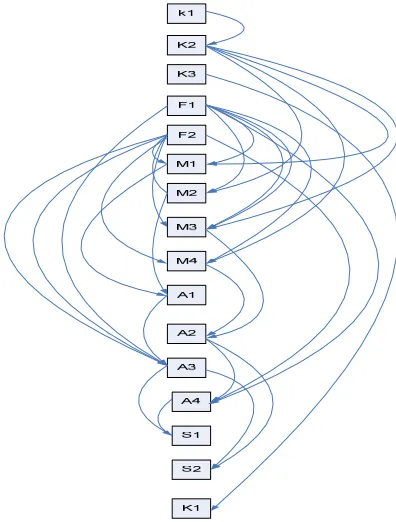
4.3: Pipelining of Algorithm
Figure 2 shows the algorithm’s operations from Table 4 with arrows showing the dependencies. The arrows of the dependencies indicate that the result of the operation at the start of the arrow is used by the operation at the end of that arrow, and it must be completed first to ensure correct data. Some arrows have a stall associated with them, specifically:
K2 – M1, M2, M3, M4
F1, F2 – M1, M2, M3, M4, A3, A4 M1, M2 – A1
M3, M4 – A2 A1, A2 – A3, A4
This means that if the operation at the start of the arrow is immediately followed by the operation at the end of that arrow, the result will be correct, but code execution will produce a stall. Thus to fully optimize the code, operations at the end of arrows with stall must be kept more than one instruction line apart.
Fig: 2: Pipelining of Algorithm
By means of windowing techniques and pipeline concept which are explained above the Fourier coefficients can be computed effectively and easily. After the FFT is calculated, we can use the complex array that resulted from the FFT to extract the conclusions.
5. Needed Software
can be downloaded through two interfaces and directly run on target. In further, the momentary result can be transmitted to PC in immediately. In the hardware specification, the maximum processing speed of ADSP TS201S can arrive on 600M Hz for core. Although the filter is floating type and processor is fixed type, the IDE can transfer float to integer for processor operation.
6.Developed Algorithm
This section describes an algorithm which is used to find the Doppler frequency from which we calculate the Relative Velocity of the target, there by the Angle between the Target paths to the source. Based upon acquired data by FPGA if pointer FIFO reads full, then FPGA gives an hardware interrupt to DSP Processor. When DSP Processor is ready to acquire data then Flag of DSP Processor will be set, in such a case FPGA dumps entire data with into DSP Processor. This Digital Data with DSP processor will be windowed using an hamming window, this windowed data is Fourier Transformed using FFT. From which magnitude of Fourier Spectrum is found. This computed magnitude is compared with threshold; the location corresponding to peak in magnitude spectrum is taken as bin number. This processes of computing magnitude of Fourier Spectrum is repeated 10 times and corresponding 10 bin numbers are found, The maximum valued bin number is selected which is used to find the frequency of target using equation 4.
These steps are shown in flow chart in figure :3 Frequency Resolution
= (Sampling Frequency) / No of FFT Points ---(4) And this Frequency Resolution
= (1024K Hz) / 1024 (512 Real + 512 Complex) points And hence Frequency Resolution = 1K Hz
From this value we calculate the Doppler frequency using DSP by predefined program based on the following formula is
Doppler Frequency = (Bin Number * Frequency Resolution)
Fig: 3: Developed Algorithm flow chart
6.1 Procedure to Calculate the Range
The total specified area will be divided into 3 sectors each one covering 120o, a transmitter and receiver are placed
in each sector. In the absence of a target in given range the frequency of a wave transmitted by the transmitter and received by receiver one and the same but where as in the presence of a target the frequency of received signal will not be same as that of transmitted. Target echo received by separate antenna, is directly down converted to base band. An IF Amplifier incorporates each sector to improve sensitivity of the Receiver. The signal at IF Port contains the target information in the form of range and Doppler. PN Sequence is 10M Hz and it is sampled at 5 times that is 50M Hz. The Doppler Frequency will vary from 10K Hz to 200K Hz and it is sampled at 5 times that is 1000 K Hz. ADC sampling frequency requirement with respect to Doppler Frequency and PN Sequence will be generated by the FPGA. PN Sequence will be generated by the FPGA. PN Sequence delay with respect to original PN Sequence will gives the delay between the transition and reception in turn will gives the range. The required range to be covered is 30 meters with 3 meters Range Resolution. Digital Correlators are implemented in the FPGA to meet the Range Resolution requirements. The ADC output is one input to the Correlators and delayed PN sequence is one more input to the Correlators. The delayed PN Sequence to be generated for the Correlators 20n sec, 40n sec, .200n sec and 300n sec, if 300n sec correlation is high, signal to be rejected. This gives the clutter rejection.
6.2 Procedure to calculate the Angle θ
From the above calculations and conclusions, using the equation 3 we calculate the angle between the Target and Source.
PN Sequence sampling Clock is 50M Hz. PN Sequence 1 frame data 155 points.
Conforming the target = Checking the PN Sequence 10 times. PN Sequence checking time
= Target Confirmation Time. = 10 * 3.1u seconds.
Once the target found data required for 1 frame 1 frame = 512 points.
From the above calculations 1 Doppler Frame acquisition time = 512u seconds Time for FFT (based on proposed method)
= 16u seconds.
After finding the target, one Doppler Frame Processing time =Data Acquisition time + Time For FFT + Other processing time.
= 512u seconds + 16u seconds + 1milli seconds.
Time for checking the each IF PN Sequence peaking = 50u seconds. Maximum time for whole processing
= 2milli seconds.
7. Results: Some representative results of our works is shown in below figures The IF Signal is shown in figure
Fig: 4.The IF Signal
Fig:6.Windowed Output
Fig:7.FFT Magnitude at 50K Hz
FFT Magnitude at 100K Hz is
8. Discussion
By implementing this proposed technique Doppler frequency of any object (Target) within the radius of 30meters can be found. This particular algorithm can be implemented within a short span of time (2mill seconds) with great peace of accuracy, Even if target is in motion within 2milli seconds (Time required for execution of algorithm) it is not possible for target to move more than 30meters in any direction and hence this opponent target can be successfully detected and necessary action can be taken. The proposed method do not have ability to locate and detect exact target(opponent),rather it considers any object with in radius of 30 meters as target and pass the same information to chief.
8. REFERENCES
[1] M. Skolnik, Introduction to Radar Systems, 2nd edition, McGraw-Hill, 1980.
[2] A.Oppenheim, R. Schafer, Discrete-Time Signal Processing, Prentice-Hall, 1989.
[5] Yi-Pin Hsu and Shin – Yu Lin, Implementation of Low-Memory Reference FFT on Digital Signal Processor.
[6] EE- 218 Technical notes on using Analog Devices DSPs, processors and development tools.
[7] Singleton, R.C., 1969, An algorithm for computing the mixed radix fast Fourier Transform. IEEE Trans. Audio Elect.,2:93-103.
[8] Kolba. D.P. and T.W. Parks. 1977, A prime factor FFT algorithm using high – speed convolution. IEEE Trans. Acoustic Speech Signal
Processing, 4: 281 – 294.
[9] Online available, TS201S DSP Processor Library Programmer’s Reference,
[10] URL: http://www.analog.com/processors/tigersharc
KODAVATI BABURAO, Asst. Prof,
ECE dept,GIET,GUNUPUR, RAYAGADA
ORISSA_765022.
T.APPARAO Asst. Prof EE dept,GIET,GUNUPUR, RAYAGADA
ORISSA_765022.
M..JAGAN MOHANA RAO Asst. Prof M.TECH HOD E&I dept
GIET,GUNUPUR RAYAGADA ORISSA_765022.