STUDY OF EFFECT OF SPEED, ACCELERATION AND
DECELERATION OF SMALL PETROL CAR ON ITS TAIL PIPE
EMISSION
Prashant Shridhar Bokare1, Akhilesh Kumar Maurya2
1 RSR Rungta College of Engineering and Technology, Kohka Road, Kurud, 490 024 Bhilai (C.G.), India 2 Department of Civil Engineering, Indian Institute of Technology Guwahati, Assam, 781039, India
Received 21 April 2013; accepted 7 August 2013
Abstract: Pollution from vehicles is due to discharges like Carbon monoxide (CO), Carbon dioxide (CO2), Hydrocarbon (HC) and Oxides of Nitrogen (NOx) through their tailpipe. Cars,
being in dominant proportions (36.5%) in Indian traffic stream with small cars above 50% in total car proportions, are the main contributors to pollutants. Literature reveals that all factors being constant, at signalized intersection, car emission rates are the function of speed and acceleration. Since it is difficult to collect speed and position data at the actual intersection, this study is conducted on link road between National Highway 31 and IIT Guwahati, India, replicating the queue leader at signalized intersection. Tailpipe emissions are measured using onboard emission measurement system and speed and position data are measured using GPS device. Study illustrates that tailpipe emissions like CO, HC and NOx are sensitive to vehicle speed at similar acceleration level. Tailpipe emission rate initially decreases with increase in speed and then increase afterwards with further increase in speed, at similar acceleration level. Emission rates are found to increase with increase in vehicle acceleration rate. It was observed that deceleration does not influence tailpipe emission of small cars.
Keywords: tailpipe emission, emission modeling, acceleration and deceleration.
1 Corresponding author: [email protected]
1. Introduction
Vehicular emissions contribute substantially to total environmental pollution for Carbon monoxide (CO), Carbon dioxide (CO2), Hydrocarbon (HC) and Oxides of Nitrogen (NOx). Measurement of vehicular emission is typically done through area wide driving cycle based models like MOBILE 5b, MOBILE 6, EMFAC, etc. The second by second data required for these models is taken from driving cycle based laboratory experiments using chassis dynamometer. However,
explaining emissions during short term episodes are termed as micro-scale emission models. Micro-scale emissions form a substantial part of total emission inventory. Micro-scale emission models are, therefore, important for evolving the traffic control strategies at road sections where short term episodes are frequent (Frey et al., 2001).
Frey et al. (2001) measured the tailpipe emissions of individual vehicles using onboard instrumentation. They considered episodic nature (nature based on temporary episodes like acceleration, breaking and deceleration) of vehicular emission. They used OEM 1000 (a five gas analyzer) to collect emission data and engine diagnostic scanner to collect engine data like speed, engine rpm, etc. at a busy arterial with signalized intersection. Authors concluded that there is a significant variation in emission of vehicles during temporary events like acceleration, deceleration and cruising. Average emission during acceleration was found to be 5 times more than idling emission for HC and CO2 and 10 times more for NO and CO. Variation of vehicular emissions with time was found to be sensitive to short term episodes like acceleration and deceleration.
Unal et al. (2004) quantified emissions at hot spots (spots where emissions are significantly high) on highway corridor using onboard emission measurement instrument. They observed that other methods of emission measurement such as chassis dynamometer; remote sensing, etc. have limitations in recording field conditions of emissions. The onboard instrument can record real world emission under any ambient traffic and roadway condition. Authors concluded that variables such as average speed, average acceleration and standard deviation
minimum speed, maximum acceleration and maximum power have significant impact on vehicle tailpipe emissions.
Wang et al. (2011) reported that vehicle speed and acceleration can be used as an input for vehicle emission models. They simulated 9.5 km freeway traffic from 15 hrs to 19 hrs to get speed trajectory, position and acceleration and deceleration. It is observed that emissions vary with variation in speed and acceleration. They concluded that emission estimates should incorporate the acceleration instead of mean speed of vehicle. Effect of acceleration on emissions is greater on lower speeds than at higher speeds. The NOx emissions suffered an increase of 34% when a correction factor for acceleration was applied.
Grace et al. (2004) reported that MOBILE5 model is widely used in emission estimation but it cannot be used in the evaluation of transportation projects improvements resulting in reduction in acceleration and deceleration. The authors included current and previous values of acceleration and deceleration along with durations of acceleration and deceleration while modeling emissions. Specific power (2 × speed × acceleration) directly determines the amount of emission. The emission models developed on the basis of these factors produced more accurate results than earlier modeling efforts. They compared emission models such as CHEM and POLY and concluded that the emissions measured by these models differ in themselves and also differed from measured values. But on evaluation, POLY model was found more reliable than other models.
consequence of vehicular emissions. They observed that most of the existing models offer simplified mathematical equations based on average link speed ignoring transient changes in speed and acceleration. They conducted various experiments to collect the data from field and chassis dynamometer for modeling vehicular energy consumption and emission rates as a function of vehicle’s instantaneous speed and acceleration. These models resulted better prediction of the vehicular energy consumption and emission rates.
Above literature indicates that the vehicular emissions can well be quantified using models based on onboard emission measurement data rather than using chassis dynamometer data for episodic nature of vehicle operation. It also shows that the vehicular emission is highly dependent on episodes like idling, acceleration, cruising and (to some extent on) deceleration. Exiting emission models like MOBILE 5b cannot be used for predicting emissions through transportation improvement projects reducing acceleration and deceleration. Further, literature yields that no such emission related study has been conducted in developing country like India. Like other developing countries, the vehicle characteristics, road features and driver habits in India are different than that reported in literature (Arasan and Koshi, 2005).
Hence this study is undertaken in India at signalized intersection (where episodes such as acceleration and deceleration are more prominent than other parts of road), to assess the sensitivity of vehicular tailpipe emission to episodes like acceleration and deceleration.
This study aims at quantifying the tailpipe emissions such as CO, HC and NOx of lead car at a signalized intersection.
2. Experimental Design and Data
Processing
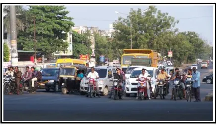
Fig. 1.
Heterogeneity and Congestion Condition in Front of the Queues at an Urban Signalized Intersection in India
2.1. Selection of Study Stretch
In order to replicate the traffic conditions of a queue leader at signalized intersection, a study stretch of following properties is chosen:
1. It should have free flow traffic; 2. It should be access controlled to avoid
any obstruction to speeding;
3. Road geometr y should be fairly straight (to have constant effect of road geometry on speed, acceleration and deceleration of vehicles);
4. Road surface should be in good condition to provide constant effect of rolling resistance.
Accordingly a study stretch is selected near main entrance of Indian Institute of Technology Guwahati (IITG), India, confirming above criteria. This road links IITG to National Highway 31.
2.2. Instruments Used
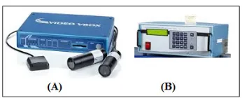
Fig. 2.
Instrumentation: (A) V-Box, (B) PEA 205, Five Gas Analyzer
2.3. Experimental Procedure
The drivers of the vehicles were asked to accelerate to their desired speed (maximum speed at which driver feel safe for a given road geometry and environmental condition; hereafter referred as maximum speed) in minimum possible time and later they were asked to decelerate till stop condition replicating lead vehicle at signalized intersection. All trips were made during free flow traffic condition. A total of 70 such trips of test car (Santro with catalytic converter) were recorded in sunny weather during November 2011.
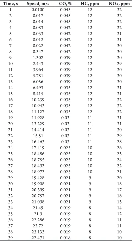
The Automotive Exhaust Gas Analyzer, PEA 205 device (Fig. 2B) was installed on back seat of car. The device was connected to laptop computer to record second by second emission data. The emission recording probe was inserted in tailpipe of the test car and the connecting pipe was attached to PEA 205 device. V-Box was installed in the test car and used to record the speed profile during all trips. The time frame synchronization of V-Box and Automotive Exhaust Gas Analyzer data was done by the time records in observed data. The speed record at a particular second is matched with tail pipe emission record at that second. A typical sample of merged data is shown in Table 1.
The observed speed and emission profiles are presented in Fig. 3. Speed profile in Fig. 3 indicates several acceleration/deceleration episodes and the episodes between one acceleration and deceleration cycle. It is seen that acceleration and deceleration episodes are repeated which are representative of acceleration and deceleration of queue leaders at signalized intersection. The maximum speed attained by any trip is 25.76 m/s (92.73 km/h).
Similarly, Fig. 3 presents the profiles of tailpipe emissions such as Carbon Monoxide (CO), Hydrocarbons (HC) and Oxides of Nitrogen (NOx). The emission profiles are superimposed on speed profile. It is seen that except for Hydrocarbons (HC), the variation in all other emissions are episodic in nature. These variations in emission profiles go with the episodes in speed, i.e. acceleration and deceleration. For Hydrocarbons (HC), initial rise in its concentration is due to un-burnt fuel due to cold start conditions. After stabilization of engine, the Hydrocarbons (HC), emission has stabilized. Salient features of speed and emissions in all trips are presented in Table 2.
highest for CO indicating higher dispersion and lowest for HC indicating lesser dispersion. This shows that the emission of CO is more sensitive to episodes like acceleration and deceleration whereas emission of HC remains more or less
unaffected due to episodes. HC emission varies initially when engine is in un-stabilized condition and emits un-burnt petrol. After stabilization engine stops emitting un-burnt petrol hence emission of HC is stabilized resulting in lesser Coefficient of Variation.
Table 1
Sample Speed and Emission Data during Acceleration Maneuver
Time, s Speed, m/s CO, % HC, ppm NOx, ppm
1 0.0100 0.045 12 32
2 0.017 0.045 12 32
3 0.014 0.045 12 32
4 0.083 0.042 12 32
5 0.033 0.042 12 31
6 0.012 0.042 12 31
7 0.022 0.042 12 30
8 0.347 0.042 12 30
9 1.302 0.039 12 30
10 2.443 0.039 12 29
11 3.964 0.039 12 30
12 5.781 0.039 12 30
13 6.056 0.039 12 30
14 6.493 0.035 12 31
15 8.415 0.035 12 31
16 10.239 0.035 12 32
17 10.943 0.035 12 32
18 11.127 0.035 12 32
19 11.928 0.03 11 31
20 13.229 0.03 11 31
21 14.414 0.03 11 30
22 15.51 0.03 11 29
23 16.463 0.03 11 28
24 17.419 0.025 10 26
25 18.486 0.025 10 25
26 18.755 0.025 10 24
27 18.492 0.025 10 22
28 18.972 0.025 10 21
29 19.428 0.021 9 20
30 19.908 0.021 9 18
31 20.399 0.021 9 17
32 20.757 0.021 9 16
33 21.098 0.021 9 15
34 21.49 0.019 8 14
35 21.9 0.019 8 12
36 22.286 0.019 8 11
37 22.72 0.019 8 11
38 23.133 0.019 8 10
Table 2
Salient Features of Speed and Emissions
Parameter Speed, m/s CO, % HC, ppm NOx, ppm
Maximum 25.76 6.93 943 735
Mean 12.49 4.52 780.9 389.97
Std.Dev 08.25 0.63 28.72 59.32
C.V. 66% 63% 13.93% 15.21%
Fig. 3.
3. Analysis and Results
Authors then calculated vehicle acceleration and deceleration using second by second speed data obtained using Eq. (1) and Eq. (2):
(1)
(2)
where; a and d are acceleration and deceleration respectively in m/s2, v
1 and
v2 are the speeds in m/s at time t1 and t2
respectively.
The speed, acceleration, deceleration and emissions such as CO, HC and NOx are then averaged over a speed range of 1 m/s (Wang et al., 2004), to get an idealized value of these parameters. Thus one idealized speed, acceleration, deceleration and emission record (CO, HC and NOx) is obtained for every 1 m/s speed range. This is done to examine average behaviour of emission with
speed, acceleration and deceleration (Rakha et al., 2000; Wang et al., 2004; Bham and Benekohal, 2001).
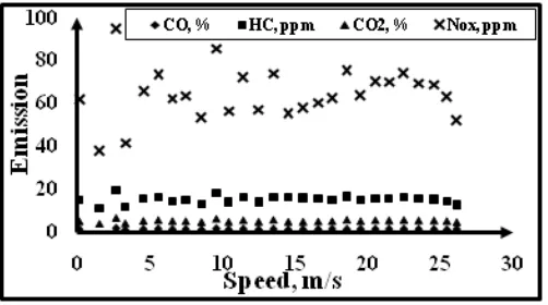
3.1. Effect of Speed and Acceleration on
Tailpipe Emission
In order to assess the effect of speed of test car on tailpipe emission, idealized emissions are plotted against idealized speed without giving consideration to acceleration or deceleration levels (Fig. 4). It is seen from Fig. 4 that there is no consistent relationship between speed and various tailpipe emissions. Similar observation is also noted by other researchers like Frey et al. (2001), Joumard et al. (1995) and Oses et al. (2002). This is due to mixing of speed records with acceleration or deceleration records. Emissions are plotted corresponding to each speed level but at particular speed vehicle may have different acceleration levels. Therefore, to segregate the acceleration effect on vehicular emission, variation of tail pipe emission with vehicular speed should be studied at a particular acceleration or deceleration level.
Hence, authors arranged speeds as per the acceleration or deceleration range and tried to find the relation between speed and emission (CO, HC and NOx) within a particular acceleration or deceleration range. For example the speed and emissions data (CO, HC and NOx) at acceleration level ≈ 1.0 m/s2 are segregated and the relationship
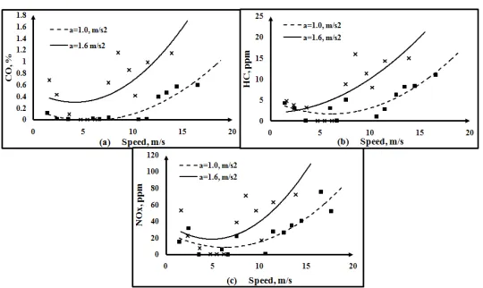
between speed and emission is tested again. It is found that at similar acceleration range, speeds and tailpipe emissions manifest a prominent relationship. Therefore, the speed and emission relationships are developed for different acceleration ranges. Figs. 5a, 5b and 5c present the relationship of CO, HC and NOx respectively, with speed at two different acceleration levels, 1.0 m/s2
and 1.6 m/s2.
It is seen from Fig. 5 that tailpipe emission rate is high at lower speed which gradually lowers with increase in speed. Later with further increase in speed emission rate increases monotonically. Similar, trend is observed for all emissions like CO, HC and NOx. At lower speed, the engine exerts more power (in first or second gear, speed 0-3 m/s) with more consumption of fuel. Higher fuel consumption results in high tailpipe emissions. As the vehicle speed advances (in second or third gear, speed 3 to 8 m/s) the power goes on reducing and hence the fuel requirement of engine goes on reducing. This reduced fuel consumption results in reduced tailpipe emission. However, with further increase in speed (in fourth or fifth
gear, speed above 8 m/s) engine consumes more fuel for speeding and results in increase in tailpipe emission. A similar behaviour is also reported by Ahn et al. (2002), Joumard et al. (1995) and Rakha et al. (2000).
The lowest tailpipe emission rate is observed at the speed range of 3 to 8 m/s (refer Fig. 5) at acceleration rate ≈ 1 m/s2 for all tailpipe
emissions. However, the speed range corresponding to lowest tailpipe emission rate reduces with increase in acceleration range. It should be noted that speed range corresponding to minimum emission are not the cruising speed of vehicle. However, this speed range corresponds to minimum emission at a particular acceleration level (like 1 m/s2 or 1 m/s2).
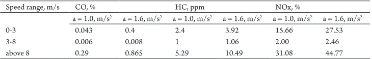
Table 3 presents average tailpipe emissions at different speed ranges and acceleration levels. It is seen from Table 3 that there is significant variation in tailpipe emission rate with different speed range and acceleration combinations. Lowest emission rate is observed in speed range of 3 - 8 m/s. It can be observed that effect of acceleration on tailpipe emissions is more prominent at higher speeds. At higher speed range (above 8 m/s), all tailpipe emission rates (CO in %, HC in ppm and NOx in ppm) are substantially high for acceleration 1.6 m/s2 than for acceleration
1.0 m/s2, as can be seen from Table 3.
This demonstrates the effect of speed and acceleration on tailpipe emission rates of test vehicle.
Table 3
Average Tailpipe Emission Rate at Different Speed Ranges and Acceleration Levels
Speed range, m/s CO, % HC, ppm NOx, %
a = 1.0, m/s2 a = 1.6, m/s2 a = 1.0, m/s2 a = 1.6, m/s2 a = 1.0, m/s2 a = 1.6, m/s2
0-3 0.043 0.4 2.4 3.92 15.66 27.53
3-8 0.006 0.008 1 1.06 2.00 2.46
Fig. 5.
Effect of Speed on Tailpipe Emission of Test Car at Particular Average Acceleration Level: (a) CO; (b) HC; (c) NOx
3.2. Statistical Comparison of Emissions
at Different Acceleration Levels
Emissions observed at various acceleration levels are statistically compared for their similarity or differences. Hypothesis is tested using t-test and the difference in means of emissions are tested using Least Significant Difference (LSD) test.
Paired ‘t’ test is used to test the means of emissions at different acceleration levels (a ≈ 1.0 m/s2 and a ≈ 1.6 m/s2). Two hypothesis
are tested − (i) null hypothesis: µ = µo− µm=
0, where µo is mean of emission at a ≈ 1.0 m/
s2 and µ
m is mean of emission at a ≈ 1.6 m/
s2 and (ii) alternate hypothesis: µ = 0. The
test statistic is calculated as follows (Eq. (3)) (Freund et al., 2011):
(3)
where, is mean of difference between µo and
µm, sd is standard deviation of difference in
paired data and n is number of data points. Hypothesis is tested for 95% confidence interval (α = 0.05, where α is significance level). One can reject null hypothesis if |t| ≥ tα/2. Table
4 presents values of t-statistics and tα/2.
Table 4
Results of Hypothesis Test
Emission |t| tα/2 Remark
CO 1.85 1.79 Null hypothesis cannot be accepted
HC 2.002 1.81 Null hypothesis cannot be accepted
NOx 2.22 1.81 Null hypothesis cannot be accepted
Table 4 indicates that the null hypothesis cannot be accepted in all cases. This indicates that there is difference in emissions
is used. LSD method performs a ‘t-test’ for pair of means using Within Mean Square as an estimate of standard deviation ‘σ2’.
It computes minimum difference at some desired significance level (generally 5% significance level). This difference is known as LSD and is computed as below (Eq. (4)) (Freund et al., 2011):
(4)
where, LSD is Least Signif icance Difference, tα/2 is α/2 tail probability
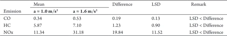
value from t-distribution and degrees of freedom, n-1, n is number observations, MSW is mean square within. LSD thus declares as significantly different pair of means for which difference between sample means exceeds LSD value. Table 5 presents means of emissions at different acceleration levels (a ≈ 1.0 m/s2and a
≈ 1.6 m/s2), their difference and LSD
values.
Table 5 indicates that in case of all emissions at acceleration level 1.0 m/s2 and 1.6 m/
s2, LSD < Difference between means.
This indicates that difference between mean emissions at different acceleration is statistically significant. This leads to a conclusion that emissions at different acceleration levels are significantly different.
3.3. Effect of Acceleration on Tailpipe
Emission
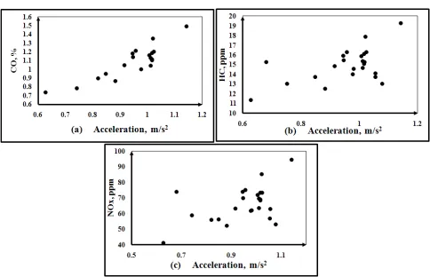
Idealized tailpipe emission (CO, HC and NOx) are plotted against average
acceleration (averaged over 1 m/s speed) and are presented in Figs. 6a, 6b and 6c. It can be observed from these figures that tailpipe emission increases with increase in vehicle acceleration. This implies lower tailpipe emission at lower acceleration and higher emission at higher acceleration. This reinforces the observation made in previous paragraph and figure.
Table 5
Means of Emissions at a ≈ 1.0 m/s2 and a ≈ 1.6 m/s2 and LSD
Mean Difference LSD Remark
Emission a ≈ 1.0 m/s2 a ≈ 1.6 m/s2
CO 0.34 0.53 0.19 0.13 LSD < Difference
HC 5.87 7.10 1.23 0.90 LSD < Difference
Fig. 6.
Effect of Acceleration on Tailpipe Emission of Test Car
3.4. Effect of Speed and Deceleration on
Tailpipe Emission
The decelerations were also averaged over 1 m/s speed range and one observation was obtained for speed, deceleration and tailpipe emission rate for every 1 m/s speed range. Various plots were drawn to explore the relationship between speed, deceleration and tailpipe emission. However, no relationship was observed between speed, deceleration and tailpipe emission. One possible reason is that the deceleration of vehicles is achieved using application of brakes. During deceleration, engine is detached from vehicle and hence doesn’t participate in the process of deceleration. Thus, tailpipe emission is unaffected by deceleration.
4. Conclusions
This study attempts to present the effect of speed, acceleration and deceleration on vehicle tailpipe emission. Test car used in this study was Hyundai Santro 2009 model (fitted with catalytic converter). Following
1. At similar acceleration level, vehicle tailpipe emission (CO, HC and NOx) is sensitive to vehicle speed. Tailpipe emission rate initially decreases with increase in speed; however, it increases afterwards with further increase in speed. Lowest tailpipe emission rate of test vehicle is observed at speed range 3-8 m/s at acceleration level 1 m/s2. Ahn
et al. (2002) reported that the emissions are lower up to speed of 5.55 m/s (20 km/h). This observation is in agreement with the lowest emission speed range of 3-8 m/s observed in this study. A similar observation is also reported by Joumard et al. (1995).
study reported by Frey et al. (2001), the minimum emission is observed at idling (at lower acceleration). At idling, since there is no power or speed requirement by engine (since there is no acceleration), the fuel consumption is minimum and hence the rate of emission is minimum. This endorses the observation by authors of present study that emission rates are lower at lower acceleration.
3. Statistically too, emissions are different at different acceleration levels.
4. R e l at ion s h ip be t w e e n v e h ic le deceleration rate and tailpipe emission was not observed.
A detailed study including different type of vehicles can be planned to develop the generalized relationship between vehicle speed, acceleration, deceleration and emission. Sensitivity of vehicular emission with its speed and acceleration/ deceleration emphasizes the need for emission consideration in designing of traffic control measures at road intersections.
References
Ahn, K.; Rakha, H.; Trani, A.; Van Aerde, M. 2002. Estimating vehicle fuel consumption and emissions based on instantaneous speed and acceleration levels,
Journal of Transportation Engineering. DOI: http://dx.doi. org/10.1061/(ASCE)0733-947X(2002)128:2(182), 128(2): 182-190.
Arasan, V.; Koshi, R . 2005. Methodology for modeling highly heterogeneous traffic flow, Journal of Transportation Engineering. DOI: http://dx.doi. org/10.1061/(ASCE)0733-947X(2005)131:7(544), 131(7): 544-551.
Belz, N.; Aultman-Hal, L. 2011. Analyzing the Effect of Driver Age on Operating Speed and Acceleration
Noise Using On-Board Second by Second Driving Data,
Transportation Research Record: Journal of the Transportation Research Board. DOI: http://dx.doi.org/10.3141/2265-21, 2265(2011): 184-191.
Bham, G.; Benekohal, R. 2001. Development, Evaluation, and Comparison of Acceleration Models. Presented at the 81st Annual Meeting of the Transportation Research Board, Washington D.C. Paper No. 02-3767. 1-42.
Carcary, W.B.; Power, K.G.; Murray, F.A. 2001. A New Driver Project. Edinburgh. 33 p.
Dey, P.P.; Chandra, S.; Gangopadhyay, S. 2008. Speed studies on two lane Indian Highways, Indian Highways, 36(6): 9-20.
Freund, R.J.; Wilson, W.J.; Mohr, D.L. 2011. Statistical Methods: Academic Press London.
Frey, H.; Rouphail, M.; Unal, A.; Colyar, J. 2001. Measurement of onroad tailpipe CO, NO and Hydrocarbon emissions using portable instrument. Presented at the Annual Meeting of Air and Waste Management Association. 1-12.
Grace, Y.; Hualiang, Q.; Teng, H.; Yu, L. 2004. Modeling Vehicle Emissions in Hot-Stabilized Conditions Using a Simultaneous Equations Model,
Journal of Transportation Engineering. DOI: http://dx.doi. org/10.1061/(ASCE)0733-947X(2005)131:10(762), 131(10): 348-359.
Joumard, R.; Jost, P.; Hickman, J.; Hassel, D. 1995. Hot passenger car emission modeling as a function of instantaneous speed and acceleration, The Science of the Total Environment. DOI: http://dx.doi.org/10.1016/0048-9697(95)04645-H, 169(1-3): 167-174.
Rakha, H.; Trani, A.; Aerde, M.; Ahn, K. 2000. Requirements for evaluating traffic signal control impacts on energy and emissions based on instantaneous speed and acceleration measurements. Presented at the
79th Annual Meeting of the Transportation Research Board,
Washington D.C. Paper No. 00-1134. 1-27.
Unal, A.; Frey, H.; Rouphil, N. 2004. Quantification of highway emission vehicle emission hot spots based on on-board measurements, Journal of the Air and Waste Management Association, 54(2): 130-140.
Wang, J.; Dixon, K.; Li, H.; Ogle, J. 2004. Normal Acceleration Behaviors of Passenger Vehicles Starting from Rest at All-Way Stop-Controlled Intersections,
Transportation Research Record: Journal of the Transportation Research Board. DOI: http://dx.doi.org/10.3141/1883-18, 1883(2004): 158-166.
Wang, M.; Daamen, W.; Hoogendoorn, S.; Arem, B. 2011. Estimating Acceleration, Fuel Consumption, and Emissions from Macroscopic Traffic Flow Data,